In the previous article in this series on AI (August 2022 issue of OSFY), we continued our discussion of matrices and linear algebra. We also discussed a few Python libraries useful in developing AI based applications, and learned to use JupyterLab to run our Python code. In this fourth article in the series on AI, we will begin exploring TensorFlow, a very powerful library used for developing AI and machine learning applications. We will also briefly discuss a few other useful libraries on the way. Later, we will discuss probability, theory as well as code. But as always, we will start by discussing a few topics that will widen our understanding of AI.
So far, we have discussed only the technological aspects of AI. What about the social aspects? Maybe, it is time to analyse the social implications of deploying more and more AI based applications. Imagine a scenario where you are applying for a job, which is processed by a group of people. They go through your resume and make a decision. In case you are not selected for the job, you can get feedback from the group that processed your application. They may even be able to convince you about the reasons for rejecting your application. Now, assume that your application is being processed by software powered with AI. Again, your application may get rejected. However, this time there is no accountability. You cannot ask an AI based software system for a feedback. So, in this scenario you are not sure whether the rejection of your application was indeed based on merit alone. This definitely tells us that in the long run we need to develop AI based applications with accountability and some guarantees, not just some results taken out of a magic box. Currently, a lot of research is trying to answer these questions.
The deployment of AI based applications also raises a lot of moral and ethical questions. Moreover, you don’t need to wait till the emergence of strong AI (also known as artificial general intelligence) to study its social impact. As an example, imagine you are driving a car through a road with hairpin bends on a rainy night. Assume that the car is running at a speed of around 100 km per hour. Suddenly, someone crosses the road. What will your response be? Since this is a thought experiment, let us make the situation even more complicated. If you suddenly apply the brakes or turn the car, your life will be in great danger. But if you don’t do this the life of the person crossing the road will be in jeopardy. For us humans, this is a split second decision and even the most selfish person may decide to save the pedestrian, because we have the trait of self-sacrifice. But how do we ever teach an AI based system to imitate this behaviour? Based on pure logic alone, self-sacrifice is a very bad choice.
Now, reimagine the same scenario with a car driven by AI based software. Since you are the owner of the car, should the AI software be trained so that your safety is the topmost priority, even to the point of utterly disregarding the safety of your co-passengers. It is easy to see that a situation where all the cars in the world are driven by such software will lead to utter chaos. Now, further assume the AI system has the additional information that the passenger riding the self-driving car is suffering from a terminal illness. With this additional information, it is logical (only to a mathematical machine, not to us, flesh and blood humans) to sacrifice the passenger for the pedestrian. I don’t want to indulge any more in this thought exercise but it will be rewarding if you could spend some time to think about the ever more complicated scenarios that may arise when decisions are made by logic-oriented machines instead of hot-blooded humans.
There are many books and articles that deal with the political, social, and ethical aspects of AI when it becomes fully operational. But I think for us mere mortals and computer engineers it would be overkill to read all of them. However, since the social relevance of AI is so important, we cannot shelve the issue that easily. To be aware of the sociopolitical aspects of AI, I suggest you watch a few movies to easily understand how AI (strong AI for that matter) may impact all of us. The masterpiece by Stanley Kubrick, ‘2001: A Space Odyssey’, is one of the first movies to depict how a superior intelligent being could look down upon us humans. This movie is one among the many in which AI decides that humanity is the biggest threat to the world and decides to destroy humans. Indeed, there are quite a number of movies where this plot is explored. But that is not the extent of it. There is a movie called ‘Artificial Intelligence’ by the great maestro Steven Spielberg himself, which explores how a machine powered with AI interacts with a human being. Another movie called ‘Ex Machina’ elaborates on this thread and deals with machines capable of artificial general intelligence. In my opinion these are all must-watch movies to understand the impact of AI.
As a final thought exercise, just contemplate roads where every car manufacturing company has its own rules and AI for self-driving cars. That will lead to complete pandemonium.
An introduction to TensorFlow
Now let us learn about TensorFlow, a heavyweight among libraries used for developing AI and machine learning based applications. Notice that, in addition to Python, TensorFlow can also be used with programming languages like C++, Java, JavaScript, etc. TensorFlow is a free and open source library licensed under Apache License 2.0, and was developed by the Google Brain team. But before we proceed any further, let us try to understand what a tensor is. If you are familiar with physics, the term tensor may not be new to you. But even if you are not familiar with the term tensor, no need to worry. Think of tensors as multidimensional arrays. Of course, this is an oversimplification. However, this simplified notion of tensors is sufficient for the time being. TensorFlow can operate on top of multidimensional arrays offered by NumPy.
First, let us install TensorFlow in JupyterLab. The kind of installation required depends on whether your system has a GPU or not. But, what is a GPU (graphics processing unit)? GPU is an electronic circuit that uses parallel processing to accelerate the speed of image processing. Though often used by gamers and designers, GPUs are an essential hardware requirement while developing AI and machine learning based applications. Unfortunately, not every GPU is compatible with TensorFlow. You need to have an NVIDIA GPU to install the GPU version of TensorFlow. Further, you need to install a parallel computing platform called CUDA (compute unified device architecture) in your system. If your system satisfies these requirements, then execute the command ‘pip install tensorflow-gpu’ on JupyterLab to install the GPU version of TensorFlow. If there is something wrong with the GPU configuration of your system, you will get the error message, ‘CUDA_ERROR_NO_DEVICE: no CUDA-capable device is detected’, when you try to use TensorFlow. If you get this error, please uninstall the GPU version of TensorFlow with the following command, ‘pip uninstall tensorflow-gpu’. Later, please install the CPU version of TensorFlow by executing the command, ‘pip install tensorflow’, on JupyterLab. Now, we are ready to use TensorFlow. Notice that, for the time being, we restrict our discussion to CPUs and TensorFlow.
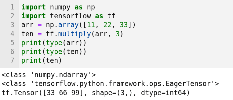
Now, let us run our first Python code powered with TensorFlow. Figure 1 shows a simple Python script and its output when executed on JupyterLab. The first two lines of code import the libraries NumPy and TensorFlow into our Python script. As a side note, if you want to display line numbers in your Jupyter Notebook cells then click on ‘View>Show Line Numbers’. Line 3 creates an array named arr with three elements using NumPy. The line of code ‘ten = tf.multiply(arr, 3)’ multiplies every element of the array arr with the number 3, and the result is stored in a variable named ten. Lines 5 and 6 print the types of variables arr and ten, respectively. From the output of the code you can see that arr and ten are of different types. Finally, line 7 prints the value of the variable ten. Notice that the shape of ten is the same as that of array arr. Also notice that ‘int64’ data type is used to represent integers in this example. Thus, with this example, it is clear that a seamless conversion between data types in NumPy and TensorFlow is possible.
A lot of operations are supported by TensorFlow. These operations become more and more complex as the size of the data being processed increases. TensorFlow supports arithmetic operations like multiply( ) (x * y) which multiplies x and y, subtract( ) (x – y) which subtracts x from y, divide( ) (x / y) which divides x by y, pow( ) (x ** y) which returns x raised to the power of y, and mod( ) (x % y) which returns x modulo y. An important point to remember is that if x and y are lists or tuples, then the operations are performed element-wise.
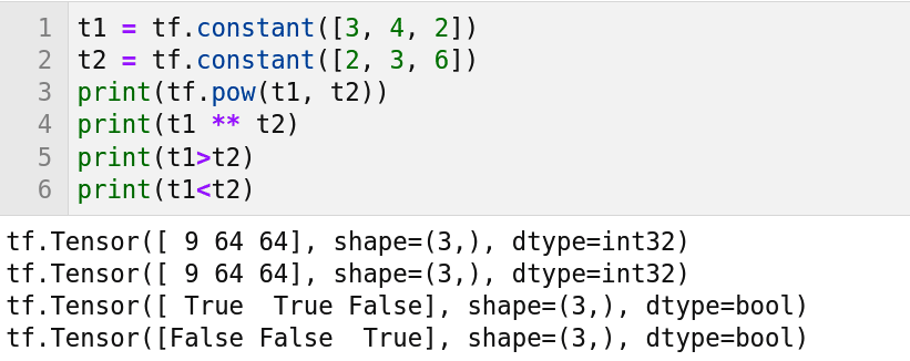
TensorFlow also supports logical, relational and bit-wise operations. Here, too, the operations are performed element-wise. Figure 2 shows a Python script in which these element-wise operations are carried out. The line of code, ‘t1 = tf.constant([3, 4, 2])’ creates a tensor from the list ‘[3, 4, 2]’ and stores it in a variable called t1. The function constant( ) is used to create a tensor from Python objects like lists, tuples, etc. Line 2 creates another tensor and stores it in a variable called t2. Both the lines of code, ‘print(tf.pow(t1, t2))’ and ‘print(t1 ** t2)’, perform an element-wise exponentiation and print the output. From Figure 2 it is clear that the result of this exponentiation, [9 64 64], is the same as [32 43 26]. The line of code ‘print(t1>t2)’ compares the elements of tensors t1 and t2 and prints results. From Figure 2, it can be verified that the output [True True False] is the result of the comparisons 3>2, 4>3, and 2>6, respectively. Similarly, the output of line 6 can also be understood.
Now, let us see one more example, this time dealing with matrices. Consider the program shown in Figure 3. Lines 1 and 3 construct two matrices named x and y. Lines 2 and 4 print the shapes of matrices x and y, respectively. From the output of the code shown in Figure 3, it can be seen that x is of shape (3, 3) and y is of shape (3, ). Further, from our earlier discussions in this series, we know that these two matrices cannot be multiplied as such.
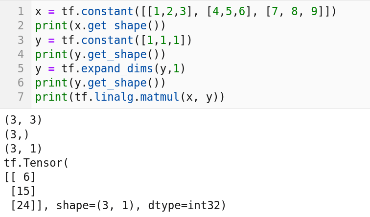
Hence, in line 5 we apply a nice technique by which the dimension of matrix y is increased by 1. In line 6, we again print the shape of matrix y. From the output, we can see that this time the shape of matrix y is (3, 1). Now matrices x and y can be multiplied. Finally, in line 7 these matrices are multiplied and the output is printed. Notice that similar operations can be performed on tensors also, and TensorFlow scales well even when the dimension of the tensor goes very high. In the coming articles in this series, we will learn more about data types and other complex operations supported by TensorFlow.
Since this is our first discussion on TensorFlow, I think I should also mention Keras. It is a software library that provides a Python interface for the TensorFlow library. In the later articles in this series, we will also get familiar with Keras.
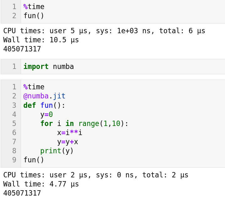
Now, we need to answer the following important question: How do we make use of a non-NVIDIA GPU? Well, there are many different ways to tap the power of these GPUs also. There are many powerful packages to do so. One such package is PyOpenCL. It allows us to use OpenCL (open computing language), a framework for writing parallel processing programs within Python. OpenCL can interact with GPUs manufactured by AMD, Arm, Nvidia, etc. But there are other options also. One such option is Numba, a JIT (just-in-time) compiler that can parallelize some parts of the Python code we have written. Thus, Numba enables the code to use our GPUs, if available. Notice that a JIT compiler is a type of compiler in which the compilation happens during execution of the code. As an example for Numba, consider the Python code shown in Figure 4. The same function called fun( ) is executed with and without using the Numba compiler. This is a simple function that finds the sum of the squares of integers from 1 to 9. Though this program is simple, on careful observation we can see that it has features that allow parallelization. From Figure 4, we can see that the code prints the same answer 405071317 on both occasions. However, we can also see that the execution time taken is different. Only half the time is taken to obtain an answer when the code is parallelized using Numba. Further, as the size of the problem being handled increases, the gap between the time taken by the parallelized and non-parallelized versions will also increase.
An introduction to SymPy
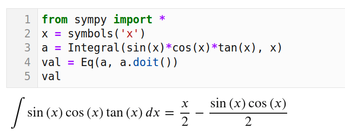
If we were discussing useful Python libraries, our discussion could have been about hundreds of such libraries. However, our discussion is about developing AI and machine learning based applications. Hence, I was a bit confused about the libraries to include in our discussion. After much deliberation, I have decided to briefly discuss SymPy. It is a Python library for symbolic mathematics. With an example, let us try to understand what symbolic mathematics is. Consider the program shown in Figure 5. It uses the function Integral( ) offered by SymPy to find the integral of ‘sin(x) X cos(x) X tan(x)’ over x. Figure 5 also shows the output of this symbolic calculation. Notice that unlike the integrate( ) function offered by SciPy, which returns numerical results, the function Integral( ) provides exact symbolic results. SymPy is useful for performing statistical operations that have high relevance in the development of AI and machine learning based applications.
In the next article in this series, we will discuss Theano, an even more powerful tool for computing mathematical expressions. Theano is a Python library and optimising compiler for evaluating mathematical expressions.
An introduction to probability
It is now time for us to have our first meeting with probability, yet another major topic of interest for AI and machine learning enthusiasts. A very detailed treatment of probability is beyond the scope of this series. I urge you to read the Wikipedia articles on ‘Probability’, ‘Bayes’ theorem’, and ‘Standard deviation’ before continuing any further. These articles are simple and easy to follow. Some of the important terms and concepts like probability, independent events, mutually exclusive events, conditional probability, Bayes’ theorem, mean, standard deviation, etc, are explained well in these articles and you will be able to follow our discussions on probability easily after reading them.
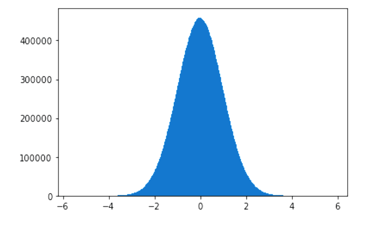
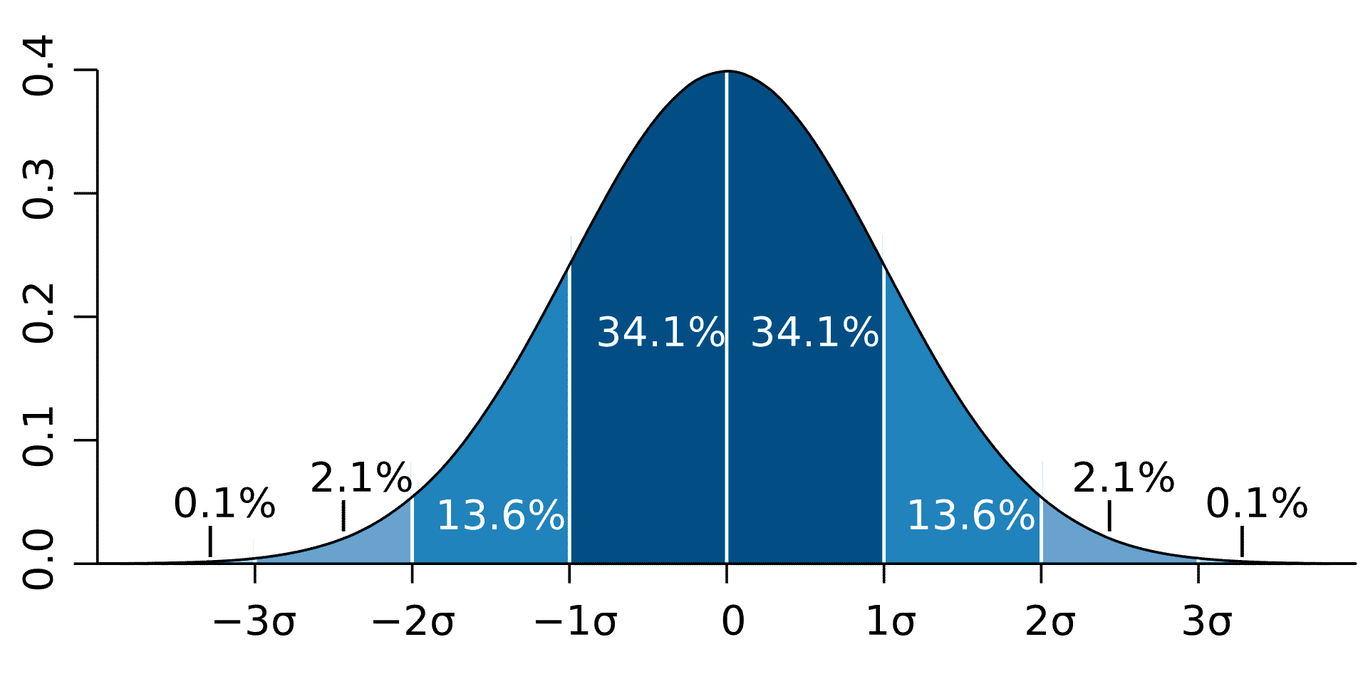
Let’s begin with probability distributions. According to Wikipedia, ‘a probability distribution is the mathematical function that gives the probabilities of occurrence of different possible outcomes for an experiment’. Now, let us try to understand what a probability distribution function is. The most famous probability distribution function is the normal distribution, often also called Gaussian distribution (named after Carl Friedrich Gauss, one of the greatest mathematicians to live on this earth). If you plot the normal distribution, you will get a bell curve. Figure 6 shows a bell curve (courtesy Wikipedia). The exact shape of the bell curve depends on the mean and standard deviation. But what does this curve signify? Let us try to understand this by analysing a natural phenomenon. A cursory search on the internet told me that the average height of an Indian man now is 1.73 metres (5 feet and 8 inches). Now, if you look around, you will see a lot of men with height very close to this figure. The chances of you observing a man who has a height below 1.42 metres (4 feet and 8 inches) or above 2 metres (6 feet and 8 inches) are very slim. Now, you go out and record the heights of say 1,000,000 men and plot a graph. Let the x-axis (horizontal axis) mark the height of a person and the y-axis (vertical axis) mark the number of samples analysed (in this case heights of 1,000,000 people). When you plot this graph, you will see a bell curve, with a few minor skews and bends. So, the mathematical equation that represents a normal distribution can easily capture natural phenomena like the heights of human beings.
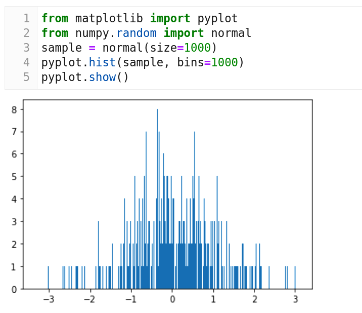
Now, let us see an example for using normal distribution. Consider the code shown in Figure 7. We use Matplotlib for plotting and NumPy for the function normal( ) which implements normal distribution. From Line 3, we can see that the sample size is 1000. Line 4 tells us that we are plotting a histogram with 1000 bins. However, if you observe the bell curve in Figure 7, this is not what we expected. This bell curve doesn’t have much similarity with the one we saw in Figure 6. What is the reason for this? Remember, our sample size is just 1000. This is like an election exit-poll where you ask the opinion of just 100 people and then make a prediction. The sample size should be sufficiently large to get a clearer picture. Figure 8 shows a bell curve when line 3 in the code in Figure 7 is replaced with the line ‘sample = normal(size=100000000)’ and the program is executed again. This time our sample size is 100,000,000 and the bell curve looks almost like the one shown in Figure 6. Normal distributions and bell curves are just the beginning. In the next article in this series we will discuss other probability distribution functions that can represent and generalise many other events and natural phenomena. Next time, we will also address the topic a bit more formally.
Now it is time for us to wind up our discussion for the time being. In the next article in this series, we will continue exploring concepts in probability and statistics. We will also install and use Anaconda, a distribution of Python for scientific computing, which is especially useful for developing AI, machine learning and data science based applications. As mentioned earlier, we will also get familiar with yet another Python library called Theano, which is used a lot in the fields of AI and machine learning. But it is also high time to do one more thing in this series. So far, we were collecting vegetables (Python libraries) and spices (mathematical concepts) to make a healthy and tasty soup (AI based applications). From the next article onwards, we will begin cooking that soup.