AI: More About Neural Networks and an Introduction to PyTorch

The previous article in this series on AI and machine learning was critical in many respects. First, we started using scikit-learn, a very powerful Python library for developing AI and machine learning based applications. Second, we deployed our first trained model. But, most important, the article introduced ChatGPT, maybe for the first time by a print magazine in India. This eighth article in the AI series talks a little more about neural networks as well as unsupervised learning, and introduces PyTorch, a very powerful framework capable of learning from data.

As mentioned in the last article, ChatGPT is a chatbot launched by OpenAI in November 2022. Within just two months of its existence, ChatGPT has created two opposing factions. One faction is supporting AI based tools like ChatGPT and waiting for a Utopian world created by AI. The other faction is worried about AI and making doomsday predictions. They fear a dystopian future — a Terminator-like scenario in which machines control humans and not the other way round. Some of the people in this faction also believe that ChatGPT will be a job killer. The jobs potentially under jeopardy according to these people include business transcription, medical transcription, copywriting, teaching, legal work, etc. But do remember that half a century ago many people believed that computers were job killers and see how mistaken they were. Some people also predict that tools like ChatGPT might be the beginning of the end for conventional search engines like Google, Bing, Baidu, etc — a belief I don’t share personally.

But what about the popularity of ChatGPT? FaceBook took 10 months to get one million subscribers in 2004. Twitter took about two years to obtain one million subscribers in 2006. Instagram was downloaded by more than one million users within 2.5 months of it being made public in 2010. All are amazing achievements. But do you know how much time ChatGPT took to obtain one million subscribers after it was made available to the public? Less than a week! Simply amazing, isn’t it? I don’t know the exact number of subscribers as of writing this article. But nowadays the services of ChatGPT are often unavailable due to the large number of users.

What about DALL-E 2, also provided by OpenAI, a tool capable of generating images from descriptions. Will normal people ever be able to distinguish between images generated by master painters and the ones generated by tools like DALL-E 2. For the sake of art, I hope at least expert curators will be able to distinguish between the two, just like a gemologist can easily distinguish between a real and a duplicate diamond, a task not easy for common people.

It is also time to think how such a ground-breaking tool like ChatGPT will affect AI related research funding. It could lead to an even bigger pile of funding in the field of AI, which might lead to further ground-breaking tools and inventions. However, such heightened expectations could also lead to disappointment and a negative reaction from the industrial giants who fund most of this research. Well, it is not safe to make predictions in times like this about the future of AI. Maybe we should ask ChatGPT to make a prediction. However, I urge you to read the Wikipedia article titled ‘AI winter’ to know more about research funding in the field of AI when exaggerated expectations are not reciprocated in reality. Also, if you still haven’t used ChatGPT or DALL-E 2, I once again implore you to try them out. You will be mesmerized. Now, let us return to our humble efforts of creating simple applications based on AI and machine learning.

Keras and neural networks

In the last article, we trained our first model using the MNIST database of handwritten digits. We have also tested our model using a few scanned images of handwritten digits. In the last article itself, we had a detailed line by line explanation of the code, except for lines 16, 19, and 20. These lines of code were the core of the model and we merely stated that fact in the last article. These three lines of code defined the properties of the neural network used in our model as well as the training parameters used. In this article, we will discuss these three lines of code in detail so that we have a clearer understanding about neural networks and their training. First, consider line 16 of the code shown below, used to develop our model. Notice that though the code spans multiple lines, syntactically it is a single statement of code.

model = keras.Sequential(
        [
keras.Input(shape=input_shape),
layers.Conv2D(32, kernel_size=(3, 3), activation=”relu”),
layers.MaxPooling2D(pool_size=(2, 2)),
layers.Conv2D(64, kernel_size=(3, 3), activation=”relu”),
layers.MaxPooling2D(pool_size=(2, 2)),
layers.Flatten(),
layers.Dropout(0.5),
layers.Dense(num_classes, activation=”softmax”),
        ]
    )

Let us briefly recall what lines 1 to 15 did to our model. First, we imported the necessary Python libraries like NumPy, Keras, etc. Then we fixed the number of classes, input shape, etc. Next, we loaded the MNIST data set and divided it into training data and testing data. Later, we checked whether a trained model exists in our system or not. We are doing this to avoid the time and resource consuming training process of a model, if a trained model already exists. If such a trained model does not exist, then the properties of a model for training are defined by the 16th line of code.

Now, let us go through that line of code shown above in detail. First, the type of neural network used is decided. Recall that a neural network has an input layer, a number of hidden layers and an output layer. Further, each layer has a number of nodes (neurons). We have defined a sequential model with the class Sequential( ) provided by the Sequential API of Keras. A sequential model is a stack of layers, where each layer has exactly one input tensor and one output tensor. This model allows us to create the neural network layer by layer. The sequential model is a relatively simple neural network model. If you want to create a more complicated neural network then use the Model( ) class provided by the Functional API of Keras. The Functional API can handle models with shared layers and multiple inputs or outputs, if required. However, I preferred the simpler sequential model.

Now, let us try to understand the input parameters given to our sequential model. The code ‘keras.Input(shape=input_shape)’ defines the shape of the input given to the input layer. In this case, the shape is (28, 28, 1) because the MNIST data set we used for training consists of a collection of 28×28 pixel grayscale images of handwritten digits. The code ‘layers.Conv2D(32, kernel_size=(3, 3), activation=”relu”)’ defines a 2D convolution layer.

By the way, what is a convolution layer? A convolution layer applies a filter to an input that results in an activation. The integer 32 in the code specifies the parameter filters, which defines the number of output filters in the convolution. The second parameter kernel_size specifies the height and width of the 2D convolution layer. Recall that we have already discussed activation functions in general and the activation function called ‘relu’ (rectified linear unit) in particular, in the 6th article in this series. Notice that a lot of other parameters can also be specified for a 2D convolution layer. But our simple example only specifies the three parameters we have discussed already. The code ‘layers.MaxPooling2D(pool_size=(2, 2))’ generates a maximum pooling layer for processing 2D spatial data. This performs a down sampling of the input along its spatial dimensions by taking the maximum value over an input window for each channel of the input. The size of the input window is specified by the parameter pool_size, which in this case is (2, 2). Now, let us go through a simple example to understand how maximum pooling works. Consider the code shown in Figure 1.

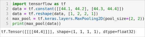
Line 1 imports TensorFlow. Line 2 defines a two-dimensional tensor named data. Line 3 reshapes the dimension of data to (1, 2, 2, 1). Line 4 uses the class MaxPooling2D to create the object max_pool. Notice that the parameter pool_size is (2, 2). Line 5 performs the maximum pooling operation on the tensor named data and prints the result. Since data is a two-dimensional tensor, only one element will be returned by max_pool. Figure 1 also shows the output of the script. It can be seen that the value returned is 44.4, the maximum value stored in the tensor named data.

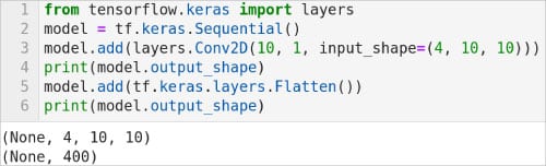
Now, let us go back to the remaining parts of the 16th line of code in our model. The code ‘layers.Conv2D(64, kernel_size=(3, 3), activation=”relu”)’ defines another 2D convolution layer of the neural network, but this time the parameter filters is specified as 64. Similarly, the code ‘layers.MaxPooling2D(pool_size=(2, 2))’ again generates a maximum pooling layer. The code ‘layers.Flatten( )’ generates a layer that gets a multidimensional tensor as input and converts it into a single dimensional tensor. For better understanding of the working of this layer, consider the code shown in Figure 2.

Line 1 imports the Layers API of Keras. Line 2 defines a sequential model. Line 3 adds a 2D convolution layer to this model by using the add( ) method. This line of code also demonstrates how a sequential model can be built layer by layer. Line 4 prints the output shape of this layer. Figure 2 shows that the output shape currently is (None, 4, 10, 10). Line 5 adds a Flatten layer. Line 6 prints the output shape of this Flatten layer. Figure 2 shows that the output shape of this layer is (None, 400). Notice that this layer does not affect the data values; it merely reshapes the data.

Now, let us consider the remaining code in the 16th line of code in our model. The code ‘layers.Dropout(0.5)’ creates a Dropout layer. This layer randomly sets input units to 0 with a frequency of rate at each step during training. This helps prevent overfitting. In simple terms, overfitting is an issue faced by mathematical models when they learn too much from the training data. This results in the model not being able to make predictions based on new data. In a Dropout layer, input data not set to 0 is scaled up by a factor of 1/(1 – rate) so that the sum over all input data remains unchanged. In our model the parameter rate is specified as 0.5. The code ‘layers.Dense(num_classes, activation=”softmax”)’ creates a densely connected neural network layer. The first parameter called units (provided by the variable num_classes in our example) defines the output dimension of this layer. Notice that in our model the variable num_classes has the value 10, because we were trying to classify the decimal digits from 0 to 9. Also, instead of ‘relu’, the activation function used is ‘softmax’, which is a slightly more complicated activation function. Please read the Wikipedia article titled ‘Softmax function’ for better understanding of this activation function. Finally, the generated model returned by the class Sequential in the 16th line of code is stored in an object named model. So altogether, our model has seven layers. Lines 17 and 18 of our code define the batch size and the epoch size of the model.

Now, consider the 19th line of code, shown below, used in developing our model.

model.compile(loss=”categorical_crossentropy”, optimizer=”adam”, metrics=[“accuracy”
])

Let us try to understand the above line of code. We need to configure the training process using the method compile( ) before we start training our model. Three parameters are given to the method compile( ). These are: loss, optimizer, and metric. Loss function is the objective that the model will try to minimise. Some of the loss functions include mean_squared_error, mean_absolute_error, mean_absolute_percentage_error, mean_squared_logarithmic_error, hinge, binary_crossentropy, categorical_crossentropy, poisson, cosine_proximity, etc. In our model, we have used the objective function called categorical_crossentropy. It is used to optimize classification models. Some of the available choices for optimizer include SGD, RMSprop, Adagrad, Adadelta, Adam, Adamax, Nadam, etc. In our model, we have used an optimizer called ‘adam’ (Adam). Adam is a first-order gradient-based optimization algorithm for stochastic objective functions. A detailed discussion of Adam is beyond the scope of our tutorial. Finally, a metric is a function that is used to measure the performance of a model. In our model, we have given ‘accuracy’ as the metric. This metric calculates how often predictions equal labels. The inclusion of this metric is the reason why we were able to print the accuracy of our model while processing the test data. In addition to the accuracy metric, there are other metrics like probabilistic metric, regression metric, image segmentation metric, etc.

Now, consider the 20th line of code shown below, used in developing our model.

model.fit(x_train, y_train, batch_size=batch_size, epochs=epochs, validation_split=0.1)

Let us try to understand the above line of code. The following parameters are passed to the fit( ) method. The variable x_train contains the training data. Training data could be either a NumPy array or a TensorFlow tensor. The variable y_train contains the target data. Target data could also be either a NumPy array or a TensorFlow tensor. Parameters to specify the batch size and the number of epochs are also passed to the fit( ) method. The parameter validation_split fixes the fraction of the training data to be used as validation data. Thus, the parameter takes a floating point value between 0 and 1. In our model, the value specified for this parameter is 0.1. After training, this model is saved in our system so that unnecessary training can be avoided in the future. Later, the test data is used to test the accuracy of the model we have trained. Finally, our model can be used to make predictions about new images of handwritten digits. With this, the discussion about our first trained model is complete.

Unsupervised learning with scikit-learn

We know that the two important paradigms of machine learning are supervised learning and unsupervised learning. Though not as popular as these two models, there are other paradigms also, like semi-supervised learning and reinforcement learning. But our discussion so far in this series was exclusively based on supervised and unsupervised learning. Though we have discussed unsupervised learning, we have given a lot of importance to supervised learning algorithms like linear regression and classification so far.

Now, it is time to discuss more about unsupervised learning, which works with unlabelled data. Just like supervised learning, in unsupervised learning also there are different algorithms like clustering, dimensionality reduction, etc. In this article, we will be focusing on clustering. Clustering is grouping a set of objects in such a way that objects in the same group are more related to each other than objects in other groups. There are many different clustering algorithms — K-Means clustering, affinity propagation clustering, mean shift clustering, spectral clustering, hierarchical clustering, DBSCAN clustering, OPTICS clustering, etc. In this article, we will be implementing K-Means clustering using the library scikit-learn.

The K-Means clustering algorithm begins by choosing K random points as cluster centres. Objects to be grouped are assigned to one of these K randomly chosen clusters. Based on the number of objects assigned to each of the clusters, new cluster centres are repeatedly calculated until the grouping of objects becomes stable. Now, let us get familiar with the Python script, shown below, implementing K-Means clustering using scikit-learn. Since the program is relatively large, a part by part explanation is given here for better understanding. Line numbers are added to the program for ease of explanation.

1. import numpy as np
2. from matplotlib import pyplot as plt
3. from sklearn.datasets import make_		   blobs
4. from sklearn.cluster import KMeans
5. X, y = make_blobs(n_samples=200, 	   	   centers=2, n_features=2, cluster_  	   std=0.5, random_state=0)
6. plt.scatter(X[:,0], X[:,1])
7. plt.show( )

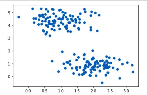
Let us try to understand the above lines of code. Lines 1 and 2 import NumPy and Matplotlib. Line 3 imports the method make_blobs(). Line 4 imports the class KMeans(). Line 5 calls the method make_blobs( ) to generate isotropic Gaussian blobs for clustering. A collection of binary data stored as a single entity is called a blob (binary large object). But what do I mean by the previous two sentences? Well, in this example, we are not using actual data; instead, we are generating sample data to test the K-Means clustering algorithm. But unlike many other occasions in this series, we are not generating random data this time. The sample data generated depends on the parameters we pass to the method make_blob( ). In this example, we are taking 200 samples (parameter n_samples) with just two centres (parameter centers). The parameter n_features determines the number of columns or features the generated data set will have. In this case it is 2. Since we are plotting the generated data in a two-dimensional plane, n_features should be at least 2. The parameter cluster_std fixes the standard deviation of the clusters. In this case it is 0.5. The parameter random_state determines the random number generation for creating the data set. The method make_blob( ) returns the generated samples (stored in array X, in this case) and the integer labels for cluster membership of each sample (stored in y, in this case). Finally, lines 6 and 7 plot and display the sample data generated in a two-dimensional plane.
Figure 3 shows this plot of the generated sample data.

Now that we have the necessary data, let us try to identify clusters from this data. The following lines of code do exactly that.

8.  kmeans = KMeans(n_clusters=2, 	    	    init=’k-means++’, max_iter=1000, 		    random_state=0)
9.  predict_y = kmeans.fit_predict(X)
10. plt.scatter(X[:,0], X[:,1])
11. plt.scatter(kmeans.cluster_centers_	    [:, 0], kmeans.cluster_centers_
    [:, 1], s=500, c=’green’)
12. plt.show( )

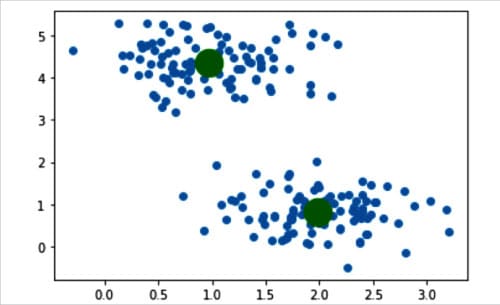
Now, let us try to understand the above lines of code. Line 8 calls the class KMeans to create an object of it called kmeans. Let us discuss the parameters passed to this class. The parameter n_clusters fixes the number of clusters to be formed as well as the number of cluster centres to be generated. In our case it is 2. The parameter init decides the method for initialisation. The two possible options for the parameter init are ‘k-means++’ and ‘random’. This parameter decides how cluster centres are identified. We chose ‘k-means++’ because it results in faster convergence while finding the cluster centres. The parameter max_iter decides the maximum number of iterations of the K-Means algorithm on a single execution. In this case, it is 1000. The parameter random_state determines the random number generated for initialising the cluster centres. In this case, it is 0. Line 9 uses the method fit_predict( ) of the class KMeans() to compute the cluster centres and also predicts the cluster to which each sample in the sample data belongs. Line 10 again plots the sample data generated. Line 11 plots the cluster centres in green colour. Finally, Line 12 displays the images plotted. Figure 4 shows this plot of the sample data generated and the cluster centres identified. Thus we have implemented our first, though simple, unsupervised learning algorithm.

An introduction to PyTorch

Now let us make ourselves familiar with PyTorch, a powerful machine learning framework based on the Torch library. Torch is an open source machine learning library and a scientific computing framework based on a programming language called Lua. PyTorch is free and open source software released under the modified BSD licence. PyTorch can work in both CPU mode and GPU mode. But in order to work with the GPU mode of PyTorch, we need to have an Nvidia graphics card and CUDA platform installed in our system. As before, the installation of PyTorch will be handled by Anaconda Navigator. Let us begin by discussing a simple Python script using PyTorch. Consider the Python script shown in Figure 5.

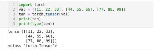
We have already discussed tensors and how they can be created using TensorFlow. We can also create tensors using PyTorch. Now, let us try to understand the Python script shown in Figure 5, which creates a tensor using PyTorch. Line 1 imports the library PyTorch. Line 2 defines a two-dimensional list named val. Line 3 converts the list val to a tensor named ten. Line 4 prints the content of the tensor ten. Figure 5 also shows the output of the script. Notice that the values in the list val remain unchanged even after getting converted to tensor ten. Finally, Line 5 prints the type of the tensor ten, which is of type torch.Tensor

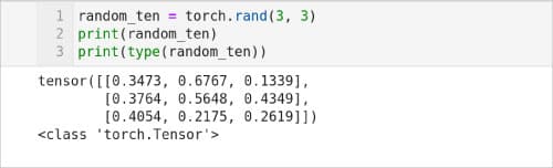
Figure 6 shows a Python script generating a tensor with random values. Line 1 of the script uses the method rand( ) to generate a 3×3 matrix and store it in a tensor named random_tensor. Line 2 prints the content of the tensor random_tensor. The output of the script is also shown in Figure 6. Notice that the content will change with each iteration because we are using the rand( ) method to generate random tensors. Finally, Line 3 prints that the type of random_tensor is also torch.Tensor.

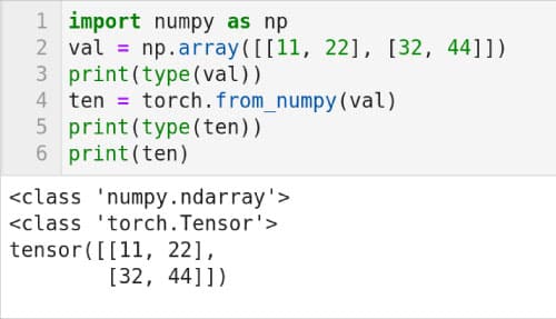
It is also possible to convert a NumPy array to a PyTorch tensor.Consider the Python script shown in Figure 7. Line 1 imports NumPy. Line 2 creates a two-dimensional NumPy array and stores it in a variable named val. Line 3 prints the type of the val. Figure 7 also shows the output of the script. It can be seen that val is of type numpy.ndarray (NumPy array). Line 4 uses the method from_numpy( ) to convert the array val to a PyTorch tensor and stores it in a variable named ten. Line 5 prints the type of the variable ten. Notice that ten is of type torch.Tensor. Finally, Line 6 prints the content of the tensor ten. The values in the tensor ten are the same as the values in the array val. We will be revisiting PyTorch in the next article in this series when we discuss natural language processing.

Now, it is time to wind-up this article. In this article, we have developed more intuition about neural networks. Further, we used scikit-learn to learn more about unsupervised learning. We also had our first interaction with PyTorch. In the next article in this series on AI and machine learning, we will continue exploring model training and neural networks. Natural language processing (NLP) is an important area in AI and machine learning. However, so far in this series we haven’t discussed anything about AI based NLP. So in the next article, we will discuss NLP using PyTorch as well as familiarise ourselves with NLTK (natural language toolkit), a Python library used exclusively for NLP.