


In the last article in this series on AI and machine learning, we started our discussion of neural networks by using TensorFlow. We also got familiar with our first data set by using Keras. In this seventh article in the AI series, we will continue exploring neural networks and the use of data sets for training models. We will also introduce yet another powerful Python library for machine learning called scikit-learn. But we will begin by discussing two sensational applications that will show us the power of AI and machine learning.
OpenAI is an artificial intelligence (AI) research laboratory which does a lot of research in the fields of AI and machine learning. Elon Musk is one of the founding members of this organisation. In November 2022, the lab launched a new online tool called ChatGPT. It is an AI chatbot that can chat like a human being. This chatbot is a large language model trained with both supervised and reinforcement learning paradigms of machine learning. ChatGPT uses OpenAI’s GPT-3.5 language model, an improved version of GPT-3 (Generative Pre-trained Transformer 3), a language model that uses deep learning to produce human-like text. I still feel the excitement I felt while using ChatGPT for the first time. The application clearly demonstrates the power of AI. The answers given by the chatbot are of high quality and often indistinguishable from a reply given by a human being. You can use ChatGPT to correct grammatical errors, rephrase sentences, summarise passages, write programs, etc. Indeed, I have rephrased many of the sentences in this article using ChatGPT. Further, I have tested ChatGPT using text with intentional grammar mistakes, not the usual ones I commit, and the corrected sentences were highly accurate. The ability to re-phrase and summarise passages was also phenomenal.
It might be even possible that programmers could solve programming puzzles within a very short time using ChatGPT. One such claim was made in a recent programming contest called ‘Advent of Code 2022’. In fact, in December 2022, just after one month of ChatGPT’s existence, Stack Overflow banned its use for generating answers.
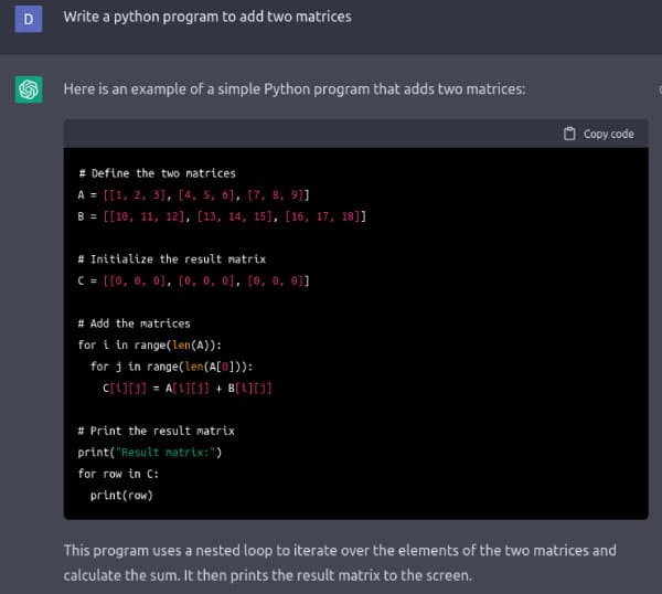
Figure 1 shows the Python program to add two matrices, written by ChatGPT. I asked for different programs in languages like BASIC, FORTRAN, Pascal, Haskell, Lua, Pawn, C, C++, Java, and even in some esoteric programming languages like Brainfuck, Ook!, etc, but ChatGPT always came up with an answer. I am pretty sure that ChatGPT is not copying the programs from some source on the Internet. Rather, I think ChatGPT is generating these answers by having a syntactic knowledge of the above-mentioned programming languages, obtained from the vast data with which it was trained. Many experts and observers are of the opinion that with the development of ChatGPT, AI has gone mainstream. Yet, the true power of ChatGPT is to be seen and analysed in the coming months and years.
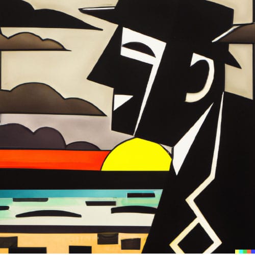
Another wonderful AI based online tool provided by OpenAI is called DALL-E 2, named after WALL-E (a cartoon robot) and Salvador Dalí (a famous painter and artist). DALL-E 2 is an AI system that can create images and art from a description given in English. The tool will generate images in different styles like oil paintings, cartoons, caricatures, realistic paintings, surrealistic paintings, mural paintings, etc. The tool can also imitate the styles of famous painters like Salvador Dalí, Pablo Picasso, Vincent van Gogh, etc. The images created by DALL-E 2 are of exceptionally high quality. I have tested the tool with the following description: ‘Cubist painting of a happy man watching sunrise near a beach’. Figure 2 shows one of the images generated by DALL-E 2 from my description. Cubism is a painting style popularised by Pablo Picasso. Ask any painter friend of yours and he or she will confirm that this indeed is a painting drawn in the Cubist style. It was quite surprising to see that software, however complicated it may be, could imitate master craftsmen like Picasso, van Gogh, Dalí, etc. I urge you to use this online tool. The experience will be quite entertaining as well as illuminating about the powers of AI. But remember that tools like ChatGPT and DALL-E 2 also bring up a lot of issues like copyright violations, copying of homework by students, etc.
Introduction to scikit-learn
Now, it is time for us to start using scikit-learn, a very powerful Python library for machine learning. This free and open-source software is licensed under the new BSD licence. Scikit-learn offers regression, classification, clustering and dimensionality reduction algorithms like support vector machines, random forests, k-means clustering, etc.
In this introductory discussion on scikit-learn, we will discuss code to implement support vector machines (SVM), a key idea in machine learning. An SVM is a supervised learning model. SVM is used for classification and regression analysis. The person behind the development of SVMs is a computer scientist called Vladimir Vapnik. He is a key figure in machine learning and, together with Alexey Chervonenkis, he proposed the Vapnik–Chervonenkis (VC) dimension, a theoretical framework to measure the capacity of a classification model.
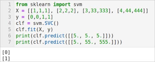
Now, consider the program shown in Figure 3. First, let us try to understand the code. The program uses SVM to classify data. Line 1 imports the svm module from scikit-learn. Notice that scikit-learn can be very easily installed by using Anaconda Navigator, as shown in the previous articles in this series. Line 2 defines a list called X which contains the training data. All the elements in X are lists of size 3. Line 3 defines a list y, which contains the class labels associated with the data in the list X. In this example, the data is classified into just two classes labelled 0 and 1. However, it is possible to classify data into multiple classes using the same technique. Line 4 uses the SVC( ) method provided by the module svm. SVC( ) method generates a support vector classifier. Line 5 uses the fit( ) method provided by the module svm to fit the SVM classifier model according to the given training data, in this case the arrays X and y. Finally, lines 6 and 7 make predictions based on this classifier. The results of the predictions are also shown in Figure 3. Notice that the classifier is able to distinguish between the two sets of data we have provided for testing.
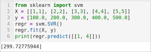
Now, let us see an example where SVM is used for regression. Consider the code shown in Figure 4. First, let us try to understand the code. Here again, Line 1 imports the svm module from scikit-learn. Line 2 defines a list called X, which contains the training data. Notice that all the elements in X are lists of size 2. Line 3 defines a list y which contains the values associated with the data in the list X. Line 4 uses the SVR( ) method provided by the module svm. This method generates a support vector regression model. Line 5 uses the fit( ) method provided by the module svm to fit the SVM regression model according to the given training data, in this case the arrays X and y. Finally, Line 6 makes a prediction based on this SVM regression model. The result of this prediction is also shown in Figure 4. There are two other methods in addition to SVR( ), LinearSVR( ) and NuSVR( ), to implement a support vector regression model. Replace Line 4 with the lines of code ‘regr = svm.LinearSVR( )’ and ‘regr = svm.NuSVR( )’, and execute the code to see the effect of these support vector regression models also.
Let us now shift our focus to neural networks and TensorFlow. But we will definitely revisit other methods provided by scikit-learn in the next article in this series when we discuss unsupervised learning and clustering.
Neural networks and TensorFlow
The deployment of neural networks is the main strength of machine learning based applications. Let us go through a few more examples from the nn (primitive Neural Net Operations) module of TensorFlow to get better familiarity with the neural network jargon. We have already seen two activation functions called ReLU (rectified linear unit) and Leaky ReLU offered by the module nn of TensorFlow. There are other activation functions also offered by the module nn. The method tf.nn.crelu( ) computes the concatenated ReLU. The method tf.nn.elu( ) computes the exponential linear function. Soon, we will use one of these activation functions while training our first model using TensorFlow and Keras.
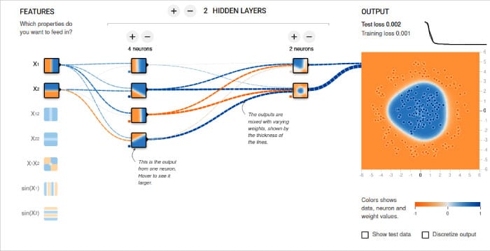
But before we move on to that section, let me share with you the details of an excellent visual tool that will help you understand the working of a neural network. This resource called ‘Neural Network Playground’ is provided by TensorFlow itself. You can visually add new neurons and new hidden layers to a neural network and then train that model. You can choose between activation functions like Tanh, Sigmoid, Linear and ReLU. Both classification and regression models can be analysed by using this tool. The effect of the training is shown as an animation. Figure 5 shows a sample neural network and the output provided by it. The tool is available online at the following URL, https://playground.tensorflow.org. This is a great resource for learning about neural networks and this might be a good time in our journey through AI and machine learning to learn more about neural networks.
Our first trained model
Now, let us continue our discussion on the MNIST database of handwritten digits, a topic which we started to learn in the last article. In this article, we will train our model completely and test it with an image of a handwritten digit. The complete program, named digit.py, is relatively large. Hence, a part by part explanation is given here for better understanding. Line numbers are added to the program for ease of explanation.
1. import numpy as np
2. from tensorflow import keras, expand_dims
3. from tensorflow.keras import layers
4. num_classes = 10
5. input_shape = (28, 28, 1)
6. (x_train, y_train), (x_test, y_test) = keras.datasets.mnist.load_data( )
Lines 1 to 3 load the necessary packages and modules. Line 4 defines the number of classes as 10 because we are trying to classify the 10 digits (0 to 9). Line 5 defines the input shape as (28, 28, 1) because the data set we are going to use is a collection of 28 X 28 pixel grayscale images of handwritten digits. Line 6 loads this data set and divides it into training data and test data. More details about this data set were provided in the previous article in this series on AI and machine learning.
7. x_train = x_train.astype(“float32”) / 255
8. x_test = x_test.astype(“float32”) / 255
9. x_train = np.expand_dims(x_train, 3)
10. x_test = np.expand_dims(x_test, 3)
11. y_train = keras.utils.to_categorical(y_train, num_classes)
12. y_test = keras.utils.to_categorical(y_test, num_classes)
Lines 7 and 8 change the pixel values of the image, which is currently in the range [0, 255], to the new range [0, 1]. The method astype( ) is used for typecasting integer values to floating-point values. Lines 9 and 10 expand the shapes of arrays x_test and x_train (changing the shape from (60000, 28, 28) to (60000, 28, 28, 1)). The lists y_train and y_test contain an array of digit labels denoting the classes. In this case, it is 10 denoting the 10 digits from 0 to 9. Lines 11 and 12 convert the lists y_train and y_test to binary class matrices.
13.    try:
14.       model = keras.models.load_model(“existing_model”)
15.     except IOError:
16.    	 model = keras.Sequential(
        	[
       keras.Input(shape=input_shape),
       layers.Conv2D(32, kernel_size=(3, 3), activation=”relu”),
       layers.MaxPooling2D(pool_size=(2, 2)),
       layers.Conv2D(64, kernel_size=(3, 3), activation=”relu”),
       layers.MaxPooling2D(pool_size=(2, 2)),
       layers.Flatten( ),
       layers.Dropout(0.5),
       layers.Dense(num_classes, activation=”softmax”),
	       ]
    	 )
17.      batch_size = 64
18.  	 epochs = 25
19.  	model.compile(loss=”categorical_crossentropy”, optimizer=”adam”, metrics=[“accuracy”])
20.   	 model.fit(x_train, y_train, batch_size=batch_size, epochs=epochs, validation_split=0.1)
21.   	 model.save(“existing_model”)
Remember that model training is a processor intensive and memory consuming operation. Thus, with lines 13 and 14, we try to load a model from the directory existing_model, if such a model is already trained and saved there. The first time you execute this code, no model is existing and hence an exception will be raised. Line 15 handles this exception by executing lines 16 to 21 which define, train and save our model. The 16th line of code (which spans over multiple lines) defines our model. The parameters given in this line decide the behaviour of our model. We are using a sequential model having a stack of layers such that each layer has exactly one input tensor and one output tensor. Our discussion of the parameters used to define the model is deferred till the next article in this series. Since neural networks are so important in machine learning, our discussion then will cover a lot of details. Until then, consider the neural network used here as a black box.
Line 17 defines the batch size as 64. This line of code decides the number of samples per batch of computation. Line 18 defines the number of epochs as 25. This value decides the number of times the entire data set will be processed by the learning algorithm. Line 19 configures the model for training. Line 20 trains the model for the given number of epochs, which in this case is 25. The detailed explanation of these two lines of code is also deferred till the next article. Finally, Line 21 saves our trained model to the directory named existing_model. You will find the model saved in this directory as a number of .pb (TensorFlow) files. Notice that lines 16 to 21 are inside the except block.
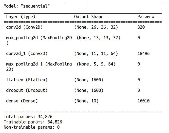
22. print(model.summary( ))
23. score = model.evaluate(x_test, y_test, verbose=0)
24. print(“Test loss:”, score[0])
25. print(“Test accuracy:”, score[1])
Line 22 prints a summary about the model trained by us. Figure 6 shows this summary of the model trained. Recall that the data set loaded in the beginning was divided into training data and test data. Line 23 uses the test data to test the accuracy of the model we have trained. Lines 24 and 25 print the details of this test.
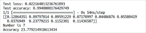
26. img = keras.utils.load_img(“sample1.png”).resize((28, 28)).convert(‘L’)
27. img = keras.utils.img_to_array(img)
28. img = img.reshape((1, 28, 28, 1))
29. img = img.astype(‘float32’)/255
30. score = model.predict(img)
31. print(score)
32. print(“Number is”, np.argmax(score))
33. print(“Accuracy”, np.max(score) * 100.0)
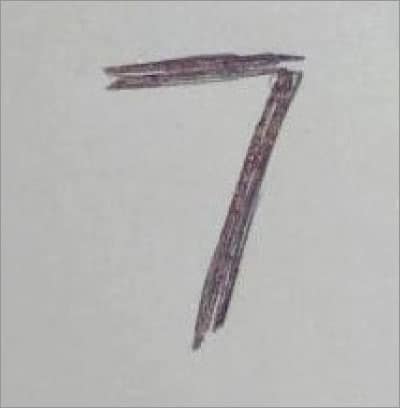
Now, it is time for us to deploy our model. I have written a few digits on paper and scanned them so that our model can use these images for classification. Figure 7 shows one of the images I have used to test our model. Line 26 loads our image after converting it to grayscale and resizing it to 28 x 28 pixels. Lines 27 to 29 do the necessary pre-processing so that the image can be given as input to our trained model. Line 30 predicts the class to which the image belongs to. Lines 31 to 33 print the details of this prediction. Figure 8 shows this part of the output of the program digit.py. From the figure it can be seen that, though the image is correctly identified as 7, the accuracy is only 23.77%. Further, from the value of the list score shown in Figure 8, it can be verified that the same number was identified as 1 with 12.86% accuracy and as 8 or 9 with about 11% accuracy. Moreover, the model even failed to identify the digit correctly on a few occasions. Though I couldn’t pinpoint any reasons for this sub-par performance, I think the relatively low resolution (28 x 28 pixel) training images as well as the quality of the scanned images I have generated could be the main contributing factors. Though not the best model available in town, we now have our first trained model based on AI and machine learning principles. Hopefully, in the coming articles in this series, we will build models capable of performing even more difficult tasks.
Now, it is time to wind-up our discussion. We have started to learn about scikit-learn in this article, a discussion we will continue in the next article in this series also. Later, we have seen more ways to deepen our understanding of neural networks. We also used Keras to train our first model and made predictions with this trained model. We will continue exploring neural networks and model training in the next article. We will also get familiar with PyTorch, a machine learning framework based on the Torch library. PyTorch is used for developing applications involving computer vision and natural language processing.
Acknowledgement: I thank my student Sreyas S. for his creative suggestions during the preparation of this article.


