


The machine learning framework outlined here converts continuous infrastructure telemetry into weekly, automated resource governance decisions, closing the gap between observability and action using entirely open source tooling. It’s particularly useful for infrastructure engineers, DevOps and SRE practitioners, database administrators, or platform engineering teams seeking to automate resource right-sizing at scale.
Your databases are drowning in their own data. They emit thousands of metrics every minute — CPU curves, memory trends, connection rates, I/O pressure — and almost none of it informs the single decision that matters most: whether those databases are the right size. Modern infrastructure operations face a persistent paradox: the systems being managed generate continuous, high-fidelity telemetry, yet provisioning decisions — the most consequential operational choice affecting both cost and reliability — are made once, at deployment time, and rarely revisited.
The consequences are well-documented. Industry benchmarks consistently report average server utilisation between 15 and 20 percent. For every five servers in a typical production fleet, the computational equivalent of four runs largely idle — provisioned against a worst case that rarely materialises, sustained by an operational culture that has no reliable mechanism to detect underutilisation and act on it.
The root cause is structural. The asymmetry of consequences in infrastructure operations creates a rational bias towards over-provisioning — under-provision and face immediate, visible incidents; over-provision and absorb invisible, silent cost. Without a system that learns from behavioural history and surfaces evidence-based recommendations, that bias persists indefinitely. So here’s a framework that closes this gap — converting operational telemetry into weekly, automated resource governance decisions using a machine learning pipeline built entirely on open source tooling.
The reactive trap: Why static thresholds fail at scale
The dominant model for infrastructure resource management is reactive: define thresholds, fire alerts when thresholds are crossed, and respond to alerts. This model has a fundamental limitation — it can only respond to states, not trajectories.
Consider a PostgreSQL database whose connection utilisation climbs steadily over four weeks: 61%, 71%, 79%, 89%. At no point does an individual reading cross a critical threshold — so no alert fires. A human who reviews dashboards at weekly intervals would need to consciously track the trend across multiple reviews to detect it. At fleet scale — tens or hundreds of database instances — that vigilance is operationally impossible. The incident that follows is framed as unforeseeable, yet the signal existed inthe data for a month before the failure. The system lacked the mechanism to learn from it.
Three specific limitations define the boundary of threshold-based alerting:
Point-in-time blindness: Alerts evaluate instantaneous or short-window metrics. They cannot distinguish a temporary spike from a sustained growth trajectory.
Single-dimension isolation: Alert rules evaluate individual metrics in isolation. They cannot model the compound risk of multiple metrics simultaneously trending towards saturation.
Static decay: Alert thresholds are set once and age poorly. A threshold calibrated for a workload six months ago may be dangerously misaligned with the workload today.
Machine learning addresses all three directly.
Architecting for behaviour, not rules
The framework given here is grounded in three design decisions that distinguish it from conventional autoscaling approaches.
Behavioural learning over rule definition: Rather than encoding human judgment into threshold rules, the framework learns decision boundaries from labelled historical outcomes. The model is not told that CPU above 85% means Scale Up — it observes thousands of instances where that metric pattern historically preceded degraded performance and infers the relationship. This makes the model’s judgment more accurate and adaptive than any rule set a human could maintain.
The four-week observability window: A rolling four week window of weekly metric aggregates is the core input structure. This horizon is long enough to capture genuine
trends and short-term seasonal patterns, short enough to remain operationally relevant for current workload characteristics, and naturally aligned with the monthly cadence at which infrastructure planning cycles operate. Instantaneous or daily readings introduce noise; annual history introduces irrelevance.
Three-state classification: Every infrastructure instance is classified weekly into exactly one of three states as given in Table 1.
This constrained output space is a deliberate design choice. Continuous scaling recommendations introduce instability and operational overhead. A weekly, three-state classification maps directly to human decision-making cadence and produces actionable outputs.
Table 1: Three-state classification output — condition and recommended action
for each state
| Classification | Condition | Action |
| Scale Down | Resources materially under-utilised across all four weeks |
Right-size to reduce cost (schedule during low-traffic window) |
| Remain | Metrics stable or trending safely within headroom |
No change — instance appropriately provisioned |
| Scale Up | Consistent upward trajectory across multiple dimensions |
Proactive scaling before saturation and incident |
Bootstrapping heuristics vs machine learning labels
A common pitfall in ML-driven infrastructure is training a model strictly on static rules (e.g., labelling training data as ‘Scale Up’ simply because CPU crossed 85%). Doing so creates a ‘surrogate model’ that merely memorises human heuristics rather than discovering true failure patterns. To avoid this, the framework uses a two-phased approach.
Phase 1: Operational bootstrapping: For initial deployment, the system can be seeded with decision boundaries derived from extensive operational experience:
- Scale Down: e.g., CPU below 40% and memory below 65% across all four weeks.
- Remain: e.g., Stable metrics, or upward trends within otherwise safe ranges (applying a conservative bias to prevent premature scaling).
- Scale Up: e.g., CPU consistently above 85% or connections consistently at or above 95% of the configured maximum.
Phase 2: True behavioural learning: As the system matures, the true machine learning labels are instead derived from actual system degradation events—such as query latency
spikes, application-side connection timeouts, or OOM kills. The Gradient Boosting classifier links the preceding four weeks of telemetry to these actual historical outcomes.
Defining the 16-dimensional observability matrix
A single vital sign tells you little. A doctor diagnosing a patient doesn’t look at heart rate alone — they read pulse, blood pressure, oxygen saturation, and temperature together, in context. Infrastructure health is no different. The model is trained not on four metrics individually, but on their joint behaviour — 16 values that together form a behavioural fingerprint no threshold rule can replicate. Four core operational metrics form the input dimensions for each classification decision:
The model is trained on the joint distribution of these four metrics over a rolling four-week window — creating a 16-dimensional input vector per instance for every classification cycle.
| Metric | Operational significance |
| CPU utilisation | Compute demand relative to provisioned capacity |
| Memory utilisation | Buffer pool saturation and working-set pressure |
| Active/Executing connections | Concurrency load relative to configured maximum (specifically isolating active execution from idle pooled connections) |
| Disk IOPS | Storage throughput pressure and I/O ceiling proximity |
This multi-dimensional structure enables the model to distinguish compound risk profiles that single-metric analysis cannot separate. A database running at 75% CPU with 20% active connection utilisation is healthy. The same CPU reading paired with 94% connection utilisation is often a precursor to an incident. The model learns this distinction directly from historical outcomes. No static threshold rule can encode it reliably.
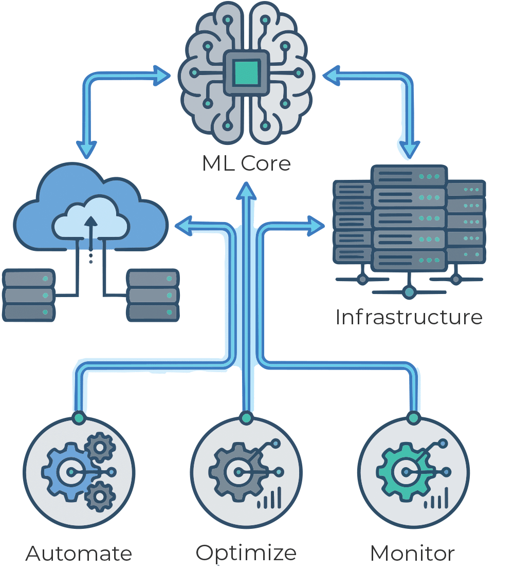
The open source engine: From telemetry to orchestration
The framework in Figure 1 is structured across four discrete layers, each with a clearly defined operational function and independent replaceability.
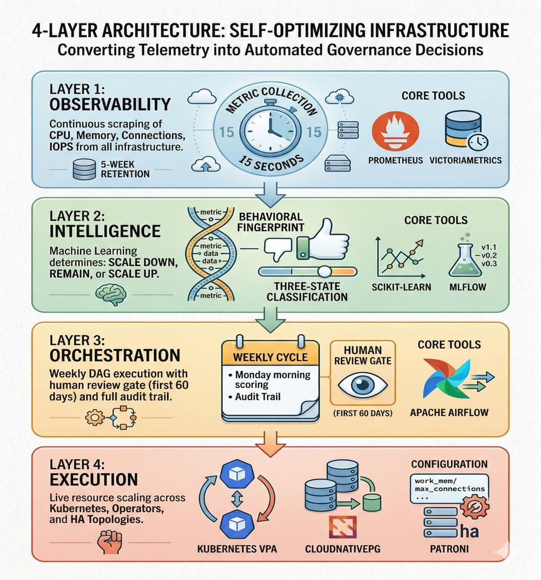
Layer 1 — Observability: Prometheus becomes the nervous system — scraping postgres_exporter and node_exporter at 15-second intervals, 24/7, without touching application code or requiring schema changes. The postgres_exporter exposes internal PostgreSQL statistics directly. Node_exporter provides host-level CPU and memory metrics. VictoriaMetrics serves as the long-term time-series store, retaining five weeks of data and answering PromQL range queries with efficient compression.
Layer 2 — Intelligence: This is where raw telemetry becomes decisions. Feature engineering produces a 16-dimensional input vector for each database instance — the behavioural fingerprint. A gradient boosting classifier trained on labelled historical data learns to generalise the classification decision. MLflow manages the model lifecycle — tracking experiments, versioning models, and maintaining an audit trail that maps every weekly recommendation to the exact model version and input features. This auditability is essential for the human review phase.
Layer 3 — Orchestration: Apache Airflow doesn’t just schedule the pipeline — it enforces the human review gate. Each stage of the weekly directed acyclic graph is independently retriable and fully logged. In the first 60 days, every recommendation lands in an engineer’s inbox before a single resource changes. This gate surfaces recommendations to the infrastructure team, builds operational confidence, and provides corrections that improve subsequent retraining.
Layer 4 — Execution: Three execution paths accommodate different PostgreSQL deployment topologies:
- Kubernetes VPA: Automatically adjusts CPU and memory resource requests on PostgreSQL pods during their next scheduled lifecycle event.
- CloudNativePG Operator: Preserves cluster topology and replication while applying resource changes through standard Kubernetes patch operations.
- Patroni REST API: Implements live configuration updates like work_mem without interruption, while staging parameters requiring restarts for the next planned maintenance window to protect high-availability integrity.
| Layer | Core tools | Function |
| Layer 1 — Observability | Prometheus, VictoriaMetrics | Metric collection (15s) and 5-week time-series storage |
| Layer 2 — Intelligence | scikit-learn, MLflow | Gradient boosting classification + model versioning and audit trail |
| Layer 3 — Orchestration | Apache Airflow | Weekly DAG execution with human review gate (first 60 days) |
| Layer 4 — Execution | Kubernetes VPA, CloudNativePG, Patroni | Live resource scaling across pod, operator, and HA topologies |
Table 2: Open source tool stack — four-layer framework summary
Real-world impact: Automating the Scale Up/Scale Down decisions
Two PostgreSQL instances drawn from production workloads illustrate the framework’s output.
Instance A — reporting database
| Week | CPU | Memory | Connections | IOPS |
| W−4 | 11% | 58% | 22% | 31% |
| W−3 | 9% | 61% | 19% | 28% |
| W−2 | 13% | 55% | 24% | 33% |
| W−1 | 10% | 57% | 21% | 29% |
Weekly metric profile — Instance A (reporting database). All four dimensions remain well within Scale Down territory across W−4 to W−1.
- Classification: Scale Down: Every metric falls within Scale Down territory across all four weeks. The model recommends reducing from 8 vCPU/ 32GB to 4 vCPU/16GB. This database was provisioned conservatively at deployment and the workload never expanded — a pattern that would have persisted indefinitely without automated detection.
- Classification: Scale Up: No individual metric has crossed a critical threshold at any point. A conventional alerting system would not have fired. The model identifies a consistent upward trajectory across all four dimensions simultaneously — a compound pattern that preceded saturation within two to three additional weeks in the training data. Proactive scaling is applied before the incident materialises.
Instance B — transactional database
| Week | CPU | Memory | Connections | IOPS |
| W−4 | 61% | 71% | 74% | 68% |
| W−3 | 66% | 74% | 79% | 71% |
| W−2 | 71% | 77% | 83% | 74% |
| W−1 | 74% | 81% | 89% | 78% |
Weekly metric profile — Instance B (transactional database). A consistent
upward trajectory across all four dimensions signals imminent saturation.
From rules to fingerprints: How the system learns over time
Model accuracy in this framework improves as a function of operational tenure. This compound improvement has three observable phases:
Month one: Recommendations reflect patterns generalised from the initial training corpus. Accuracy is meaningful but imprecise at the instance level.
Month three: With twelve weeks of inference history, the model begins developing behavioural fingerprints — patterns unique to each instance. The reporting database that spikes every Friday at 15:00; the analytics instance that peaks during monthend batch runs. By month three, the model knows that a Monday morning spike on Database is anomalous — because the training data shows Friday is its normal peak.
Month six: Seasonal patterns, sustained growth trajectories, and workload anomalies are fully internalised. The model reliably distinguishes a temporary spike from a structural demand change. Recommendation accuracy at this tenure supports confident transition to full autonomous execution.
This compounding dynamic separates ML-based infrastructure governance from static automation, creating a structured pathway from human-reviewed reports to autonomous resource management.
Beyond PostgreSQL: Adapting the pattern for Redis, Kafka, and Elastic
The ‘observe-learn-classify-act’ pipeline is infrastructureagnostic; while specific metrics and scaling endpoints vary by technology, the underlying ML architecture remains identical.
- Redis: Uses memory and eviction patterns to scale up before cache hits are impacted or scale down during low use.
- Kafka: Monitors consumer lag and replication to predict broker exhaustion, preventing data pipeline outages.
- Elasticsearch: Analyses heap and shard patterns to trigger proactive rebalancing or node additions before query latency degrades.
In all scenarios, the Airflow DAG, scikit-learn classifier, and MLflow registry require zero modifications—only Prometheus targets and execution layers change.
Day One deployment: Building your minimum viable pipeline
You don’t need to solve the entire problem on Day One. The goal is to make the invisible visible. By the end of the day, you’ll have a working data pipeline and — for the first time
— a weekly report showing you which of your databases are quietly wasting money and which are quietly heading towards an incident. A minimum viable deployment requires
just three components:
Metrics pipeline: Prometheus with postgres_exporter and node_exporter pointed at target instances, and VictoriaMetrics configured for five-week retention.
Weekly scoring job: A Python script that queries VictoriaMetrics and outputs a classification — initially using hardcoded heuristics, replaced with the trained ML model once sufficient labelled history is available.
Human review step: Recommendations delivered by email each Monday morning. No automated execution.
This phase validates the data pipeline and begins building the labelled training dataset that makes the model smarter over time. Automation is introduced incrementally — never all at once. Scale Down actions carry the lowest operational risk and are the appropriate first target: incorrect recommendations are reversible.
Scale Up automation follows with a lightweight approval gate. Full autonomous execution is appropriate once model accuracy demonstrates consistent reliability. The path from human-reviewed reports to autonomous governance is measured in weeks, not months.
The data required to make intelligent infrastructure decisions already exists in every PostgreSQL deployment. The gap is the absence of a learning system that converts observability into governance action. The framework presented here closes that gap using open source tooling, a four-week observability window, and a classification model that improves continuously.
Infrastructure managed by this framework reduces waste, prevents incidents, and compounds in accuracy. It is a generalised blueprint for autonomous infrastructure governance — applicable to any workload that generates behavioural telemetry. The organisations that deploy this capability build infrastructure that earns the right to manage itself.


