


In the previous article in this series (published in the January 2026 issue of OSFY), we concluded our discussion of cybersecurity and the implementation of various cybersecurity algorithms using SageMath. We will now explore SageMath libraries and packages that can be applied to the field of mathematics known as number theory.
Number theory has wide-ranging applications in computer science, including cybersecurity, algorithm design, random number generation, error-correcting codes, computer graphics, machine learning, artificial intelligence, and blockchain. The following quote by the famous mathematician Carl Friedrich Gauss — often called the ‘Prince of Mathematics’ — highlights the importance of number theory: “Mathematics is the queen of the sciences, and number theory is the queen of mathematics.” (In Gauss’s time, number theory was commonly referred to as arithmetic.)
Let us begin by discussing a fundamental requirement in computation: the ability to store very large integers without overflow. As we already know, Python can handle arbitrarily large integers, and SageMath inherits this capability. Let us look at a few examples that demonstrate how SageMath works with extremely large numbers. As in our previous articles involving heavy mathematical computations, we will use CoCalc rather than running the code locally on our systems. Consider the SageMath code shown below.
n = 10^1000
print(n)
In the above code the integer 10^1000 — which, by definition, has no fractional part — is stored in the variable n. The caret symbol (^) denotes exponentiation, and SageMath stores the resulting value exactly, without any loss of precision. However, I will not display the full number here, as it would occupy at least one paragraph. Let us instead turn to even larger numbers, expressed using notations such as Knuth’s up-arrow notation (↑), introduced by the famous computer scientist Donald Knuth.
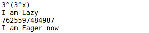
Let us now understand Knuth’s up-arrow notation. Exponentiation is written as a↑b, which corresponds to a^b in SageMath. For example, 3↑4 = 34 = 81. Now consider the double-arrow operator (↑↑). The expression 3↑↑3 represents a power tower: 3^(3^3) = 3^27 = 7625597484987. From this, one can imagine how a number such as 3↑↑10 would behave — it is a tower of ten 3’s stacked in exponent form. Mathematics contains notations that grow even faster, such as Graham’s number, which describes quantities far beyond everyday intuition. To work with such astronomically large expressions, SageMath relies on a technique called lazy evaluation. Lazy evaluation means an expression can be stored symbolically without being fully computed until its value is explicitly required. The SageMath program ‘exp43.sage’ (line numbers included for clarity), shown below, evaluates the expression 3↑↑3.
1. # 3↑↑3
2. var(‘x’)
3. expr = 3^(3^x)
4. print(expr)
5. print(“I am Lazy”)
6. print(expr(x=3))
7. print(“I am Eager now”)
Now, let us try to understand the working of the program. Line 1 is just a comment that tells us what we are going to evaluate. Line 2 declares x as a symbolic variable in SageMath. Line 3 creates a symbolic expression, not a number. SageMath stores the expression ‘3^(3^x)’ as a formula. Line 4 prints this symbolic expression. Line 5 is just a message that highlights that, up to now, nothing has been computed. Line 6 performs the actual numeric evaluation and prints the result. Finally, Line 7 prints a message confirming that we forced an evaluation to obtain a concrete result and that laziness has ended. As we can see from the message, the opposite of lazy evaluation is called eager evaluation (also called strict evaluation), where the expression is evaluated immediately to obtain the numerical result. Upon executing the program ‘exp43.sage’, the output shown in Figure 1 is obtained.
The SageMath program ‘lazy44.sage’, shown below, demonstrates a simple way to implement lazy evaluation when working with Knuth’s up-arrow notation such as 3↑↑10.
class Tetration:

def __init__(self, a, n):

self.a = a

self.n = n

def __repr__(self):

return f”{self.a}↑↑{self.n}”

t = Tetration(3, 10)

print(t)
When executed, the program simply prints ‘3↑↑10’ on the terminal. At first glance this appears trivial — the program stores and returns a string representation rather than computing a number. However, this idea is powerful: instead of attempting to evaluate an astronomically large quantity, we store its symbolic form. Such symbolic representations allow SageMath to manipulate expressions that are far too large to compute explicitly, which is the essence of lazy evaluation in practice.
Let us now examine why SageMath is so efficient and powerful when it comes to integer manipulation. Much of this strength comes from the number-theoretic libraries it builds upon — such as FLINT, GMP, PARI/GP, ECM, and NTL — which we discussed in earlier articles in this series. In this article, we will introduce another important component that contributes to SageMath’s power: the GNU Multiple Precision Floating-Point Reliable Library (GNU MPFR).
The need for a library like MPFR arises from a fundamental question closely tied to number theory: how floating-point numbers are represented in a computer. It is easy to see that not all real numbers can be stored with absolute precision. To illustrate, consider writing the number 1/3 in decimal form as 0.333…. Even if you had a million notebooks, you could keep writing 3s forever and still never reach the end. A computer faces the same limitation: it has only a finite amount of memory, so it must stop after a fixed number of digits and round the result.
The situation becomes even more striking in binary. Many simple decimal fractions cannot be represented exactly in base 2. For example, the decimal number 0.1 has an infinite repeating expansion in binary: 0.110 = 0.00011001100110011…2. Since the expansion never terminates, a computer stores only a truncated approximation. As a result, calculations involving 0.1 may introduce tiny rounding errors. For instance, in many programming languages including Python the expression ‘0.1+0.2’ does not produce exactly 0.3, but a nearby value such as 0.30000000000000004. Libraries like MPFR are designed to manage such issues by providing well-defined, high-precision floating-point arithmetic with controlled rounding, which is essential in important numerical and number-theoretic computations.
Now, let us see how MPFR handles this issue. But before we proceed let us execute the statement ‘0.1+0.2’ on SageMath without using the additional features provided. Upon execution of this statement, we can verify that the output displayed is 0.300000000000000. So, even without using any special libraries SageMath outperforms Python as far as handling floating point numbers. Now, let us consider the following code where MPFR is used to arbitrarily increase the precision of floating point arithmetic. The SageMath program ‘mpfr45.sage’ (line numbers included for clarity), shown below, demonstrates how floating point arithmetic is handled by MPFR.
1. R = RealField(100)

2. print(R(1) / R(3))

3. R = RealField(200)

4. print(R(1) / R(3))

5. print(R(0.1) + R(0.2))

6. print(R(“0.1”) + R(“0.2”))

7. print(R.pi( ))

8. R = RealField(100, rnd=’RNDN’)

9. print(R(1)/3)

10. R = RealField(100, rnd=’RNDD’)

11. print(R(1)/3)

12. R = RealField(100, rnd=’RNDU’)

13. print(R(1)/3)

14. R = RealField(100, rnd=’RNDZ’)

15. print(R(1)/3)
Now, let us try to understand the working of the program. Line 1 creates a real number field R with 100 bits of precision using MPFR through SageMath. It tells SageMath to use high-precision floating-point numbers instead of the usual double precision. Line 2 computes and prints the value of 1/3 in that 100-bit precision field. Line 3 redefines R with higher precision (200 bits), and line 4 prints 1/3 again, now with greater accuracy, illustrating how precision can be increased without changing the computation itself. Line 5 adds 0.1 and 0.2 after converting them from machine floating-point numbers into the high-precision field, which may still carry tiny binary rounding errors from their original representation. Line 6 adds the numbers using string input “0.1” and “0.2”, forcing SageMath to interpret them as exact decimals before conversion, thereby avoiding prior floating-point error. Line 7 prints the constant π computed to 200-bit precision using MPFR. Line 8 creates a 100-bit field with rounding mode ‘round to nearest’ (RNDN), and Line 9 prints 1/3 under this rounding rule. Lines 10 to 15 repeat the computation of 1/3 using different rounding modes: RNDD rounds downward, RNDU rounds upward, and RNDZ rounds towards zero. Together, these lines demonstrate how SageMath utilises MPFR’s ability to control both precision and rounding behaviour, which is essential for reliable high-precision numerical work. Upon executing the program ‘mpfr45.sage’, the output shown in Figure 2 is obtained.
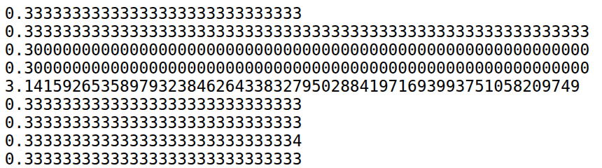
The last four lines in Figure 2 show the output produced using the four MPFR rounding modes. From this output alone, the distinction between RNDD and RNDZ may not be immediately apparent. The code snippet below clarifies the difference, demonstrating that these two modes behave differently only for negative numbers.
R = RealField(50, rnd=’RNDD’)
print(R(0.9))
R = RealField(50, rnd=’RNDZ’)
print(R(0.9))
R = RealField(50, rnd=’RNDD’)
print(R(-0.9))
R = RealField(50, rnd=’RNDZ’)
print(R(-0.9))
Upon execution, the output shown below is produced. From this output, it is evident that rounding down and rounding towards zero differ when negative numbers are processed.
0.89999999999999
0.89999999999999
-0.90000000000001
-0.89999999999999
In addition to providing precise representations of integers and floating-point numbers, MPFR implements a wide range of advanced numerical functions that are particularly valuable in number-theoretic computations. The SageMath program ‘functions46.sage’ (line numbers included for clarity), shown below, demonstrates the use of several of these MPFR functions.
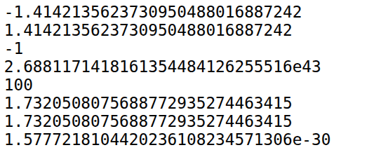
1. R = RealField(100)

2. x = -R(2).sqrt()

3. print(x)

4. print(abs(x))

5. print(x.sign())

6. print(R(100).exp())

7. print(x.prec())

8. x = R(3).sqrt()

9. print(x)

10. print(x.nextabove())

11. print(x.nextabove() - x)
Now, let us try to understand the working of the program. Line 1 creates a real-number arithmetic system with 100 bits of precision. Line 2 converts the integer 2 into a 100-bit real number and computes its square root inside that high-precision system. Then the result is negated. Line 3 prints the value of x, which is −√2, rounded to the number of decimal digits SageMath chooses to display. Line 4 prints the absolute value of x. Since x is negative, abs(x) removes the sign and prints a positive approximation of √2. Line 5 prints the sign of the number (-1 if negative, 0 if zero, and +1 if positive). Since x is −√2, the output is -1. Line 6 converts 100 into a high-precision real number and computes e100, the exponential function. The result is a very large number printed using 100-bit precision. Line 7 prints the precision of x, confirming that it is stored with 100 bits of precision. Line 8 replaces the old value of x with a new high-precision number (√3). Line 9 prints the high-precision decimal approximation of √3. Line 10 prints the next representable floating-point number greater than x. It is the smallest number larger than √3 that can be stored in the 100-bit system. Line 11 prints the difference between √3 and the next representable number. That value is the ULP (Unit in the Last Place) at √3 — the smallest spacing between numbers at that magnitude.
When the program ‘functions46.sage’ is executed, the output shown in Figure 3 is produced. The sixth and seventh lines display the approximate value of √3 and the next representable value greater than √3. At first glance, this result appears surprising because both numbers are printed identically. However, they are not equal internally. The difference becomes evident in the following line of the output, where the subtraction of the two values yields a nonzero result — a very small fraction representing the spacing between adjacent floating-point numbers. This example illustrates the care that SageMath and the MPFR library take in preserving numerical precision. Even when two values appear identical when printed, the system maintains their exact internal distinction at the level of machine precision.
What we have discussed here is only the tip of the iceberg. MPFR is a powerful library with extensive capabilities, and it is well worth exploring further. We now turn to another important topic in number theory: primality testing.
In the previous articles in this series, where we discussed cybersecurity related topics, we performed prime factorization and primality testing. However, we did not specify which primality testing algorithm was used. Broadly, primality testing algorithms are classified into two types: deterministic and probabilistic. Deterministic algorithms always produce a correct result, but they are often slower than many probabilistic algorithms. Probabilistic algorithms, on the other hand, may occasionally produce an incorrect result. A probabilistic primality test will never report a prime number as composite. However, it may classify a composite number as a probable prime.
Let us now examine some important deterministic primality testing algorithms. Sieve-based methods form a family of algorithms that are primarily used for generating all prime numbers up to a given limit, rather than testing the primality of a single very large integer. Among these, the most famous is the Sieve of Eratosthenes, named after the Greek mathematician Eratosthenes, who is also credited with the first known measurement of the Earth’s circumference.
The sieve works by systematically eliminating composite numbers. First, list all integers from 2 up to the desired limit. Circle the first number (2) and cross out all its multiples. Move to the next uncrossed number (3), circle it, and again eliminate its multiples. This process continues, advancing to the next uncrossed number each time. Once all multiples of primes up to √n have been removed, the numbers that remain uncrossed are precisely the prime numbers.
Modern sieve-based techniques, such as segmented sieve, are used internally in SageMath through high-performance numerical libraries such as GMP and PARI/GP. The following code generates and prints all prime numbers less than 1000 by leveraging these optimised libraries.
n = primes(1000)
for i in n:
print(i)
Although it is not used in SageMath, it is important to mention another landmark deterministic primality testing algorithm: the AKS primality test, developed by Manindra Agrawal, Neeraj Kayal, and Nitin Saxena at the Indian Institute of Technology Kanpur. Their groundbreaking paper, ‘PRIMES is in P’, proved for the first time that primality testing can be done in deterministic polynomial time. The work was widely celebrated and received both the Gödel Prize and the Fulkerson Prize in 2006, recognising its profound impact on theoretical computer science and discrete mathematics. It remains one of the most significant achievements by Indian computer scientists in modern times.
Let us now discuss some probabilistic primality testing algorithms. Important members of this class include the Fermat test, the Solovay–Strassen test, the Miller–Rabin test, and the Baillie–PSW test. The Fermat and Solovay–Strassen tests are primarily of theoretical and academic interest, whereas the Miller–Rabin and Baillie–PSW tests are widely used in practical applications. A full technical treatment of these algorithms is beyond the scope of this series; however, it is useful to understand how the confidence level of probabilistic tests can be amplified. Most probabilistic primality tests guarantee that the probability of incorrectly declaring a composite number to be prime is at most 1/4 in a single run. If the same test is repeated independently and a number is reported as prime each time, the error probability decreases multiplicatively. For example, running the test twice reduces the error probability to 1/4 × 1/4 = 1/16. By repeating the test many times, the probability of mistakenly accepting a composite number as prime can be made arbitrarily small, though never exactly zero. Importantly, these algorithms are designed so that they never classify a true prime as composite; the only possible error is falsely labelling a composite number as prime.
Let us now examine how SageMath allows the user to choose between deterministic and probabilistic primality testing algorithms. When the function is_prime( ) is used in SageMath, either a deterministic or a probabilistic algorithm is selected internally, depending on the size of the number being tested and the level of confidence required in the result. The SageMath program ‘primality47.sage’ (line numbers included for clarity), shown below, demonstrates how the programmer can control the algorithm used in the background for primality testing.
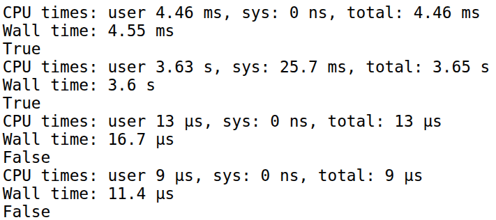
1. n = random_prime(2^1024)

2. %time n.is_prime(proof=False)

3. print(n.is_prime( proof=False))

4. %time n.is_prime(proof=True)

5. print(n.is_prime(proof=True))

6. n = 100

7. %time n.is_prime(proof=False)

8. print(n.is_prime(proof=False))

9. %time n.is_prime(proof=True)

10. print(n.is_prime(proof=True))
Now, let us try to understand the working of the program. Line 1 generates a random prime number less than 21024. Notice that this is a very large (approximately 1024-bit) prime number. When Line 2 is executed, SageMath delegates the computation to the PARI/GP library. PARI/GP runs the Baillie–PSW primality test (a combination of the Miller–Rabin and Strong Lucas primality testing algorithms) to determine whether the given number is prime. If the algorithm returns False, the number is composite (with 100% certainty). If it returns True, the number is classified as probably prime—that is, it is not a proven prime, and there remains a very small probability that it could be composite. The magic command %time measures how long the computation takes. Line 3 prints the result of the probabilistic test. Line 4 runs a deterministic primality testing algorithm because the option proof=True is specified. In this case, SageMath uses either the APR-CL test (Adleman–Pomerance–Rumely–Cohen–Lenstra) or ECPP (Elliptic Curve Primality Proving). We will not discuss these algorithms here, as they are advanced topics beyond the scope of this series. The time taken for this operation is also measured using %time. Line 5 prints the result of the deterministic test. Lines 6 to 10 perform the same operations on a small composite number (in this case, 100).
When the program ‘primality47.sage’ is executed, the output shown in Figure 4 is obtained. From the first six lines of the output, we can verify that the large number is correctly identified as prime by both the probabilistic and deterministic algorithms. The timing data also shows that the probabilistic algorithm is approximately 791 times faster than the deterministic algorithm for this large input. Lines 7 to 12 confirm that both algorithms correctly classify the number 100 as composite. Interestingly, in this case the deterministic algorithm outperforms the probabilistic one. This highlights an important practical observation: for relatively small inputs, deterministic algorithms may be preferable. They can be faster in this situation and, moreover, provide a guaranteed correct result without relying on probabilistic confidence.
Now it is time to wrap up our discussion. In this article, we have explored several important topics in computer science that are rooted in number theory. Precise integer and floating-point operations are essential in nearly all real-world applications. Even small computational errors can lead to catastrophic consequences. For example, the failure of the Ariane 5 rocket launched by Arianespace on June 4,1996, was caused by an integer overflow error, resulting in a loss of more than US$ 370 million. This highlights the critical importance of accurate numerical computation. Likewise, primality testing plays a vital role in many real-world applications, particularly in areas such as cryptography and security. Given the fundamental importance of number theory, we will explore it further in the next article in this series.


