


Discover the concepts of drift and data skew, and explore online monitoring techniques that keep your machine learning model relevant.
In traditional software engineering, a deployment is often the end of the primary development cycle. If the unit and integration tests are passed, the software is generally expected to function until the code changes. Machine learning (ML) is fundamentally different. An ML model is a mathematical representation of a specific period. The moment it is deployed, it begins a journey towards obsolescence.
Unlike a database that crashes or an API that returns a 500 error, a decaying ML model will still return a prediction. It will still provide a ‘probability score’. It looks healthy on your infrastructure dashboard, but the business value it provides is evaporating. This is why continuous monitoring is not an ‘add-on’ for MLOps; it is the heartbeat of the production lifecycle. Without it, you are flying blind in a changing world.
Understanding drift and skew
To monitor effectively, we must first categorise how models fail. In the world of MLOps, there are three distinct types of ‘distance’ between what the model expects and what it is really seeing.
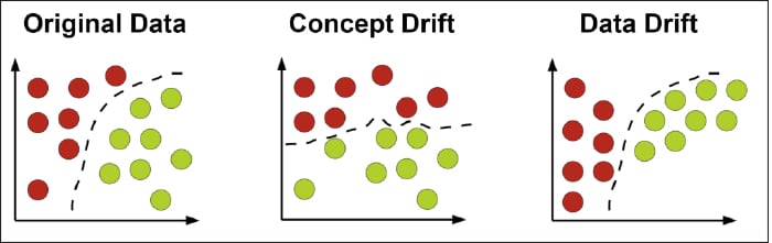
Data drift (covariate shift)
Data drift occurs when the statistical distribution of the input features changes over time. The model’s internal logic remains ‘correct’ based on its training, but it is being asked to make predictions on data it has never seen before.
- The ‘new user’ problem: A fintech model trained on urban professionals is suddenly deployed in a rural market. The income levels, spending habits, and credit histories look different. The model hasn’t ‘failed’, but it is operating outside its ‘zone of competence’.
Concept drift (posterior probability shift)
This is the most dangerous form of decay. Concept drift occurs when the relationship between the input and the target variable changes. Even if the input data looks exactly like the training data, the meaning of that data has shifted.
- The post-pandemic shift: Consider a model predicting consumer demand for travel. Before 2020, a ‘low-cost flight’ may have been a strong predictor of a ‘guaranteed booking’. After 2020, the concept of ‘safety’ or ‘cancellation flexibility’ became more important than price. The features didn’t change, but the world’s behaviour did.
Training-inference data skew
While drift happens over time, data skew is a structural discrepancy. It is often caused by technical debt or architectural flaws.
- Feature engineering mismatch: If your training pipeline uses a Python library to calculate a ‘7-day rolling average’ and your production C++ backend uses a slightly different windowing logic, you have skew.
- Data leakage: A classic mistake where a feature that is only available after the event (e.g., ‘total call duration’ for a churn model) is accidentally used in training.
Common drift detection methods
When monitoring models in production, we can’t rely on gut feel or visual inspection alone. Small shifts may look harmless but compound over time, while large shifts may be obvious but hard to justify without evidence. What we need is a systematic way to answer one question: Does today’s data behave differently from what the model was trained on?
Drift detection methods give us objective signals to answer this by comparing the current data distribution to a reference (training or baseline) distribution.
Distribution comparison (statistical distance)
At a high level, these methods ask: How different are two distributions?
Numerical features: For continuous or numerical variables (e.g., price, latency, session duration), the Kolmogorov–Smirnov (K-S) Test is commonly used, which compares the shape of two distributions, not just their averages. It is non-parametric, meaning it makes no assumptions about normality. The output is a single distance score representing the maximum separation between the two distributions. If this distance exceeds a threshold, we conclude that the feature has statistically drifted.
Categorical features: For discrete features such as country, device type, or product category, numerical distance tests are not applicable. We can either use the Chi-Squared Test or the Jensen-Shannon Divergence. The Chi-Squared Test checks whether category frequencies have changed more than expected by chance. The Jensen-Shannon Divergence (JSD) measures how similar two probability distributions are, in a bounded and symmetric way.
Population Stability Index (PSI)
While statistical tests tell us whether a change is significant, teams often want a single, easy-to-interpret score. This is where PSI is widely used in industry. However, its thresholds should be treated as a guideline.
The commonly used ranges are:
- PSI < 0.1 (no change)
- 0.1-0.25 (moderate drift)
- 0.25 (significant drift)
In high-risk systems (fraud detection, medical models, credit underwriting), even small PSI values may warrant investigation. In noisy consumer data (clickstream, marketing), larger PSI values may be acceptable. The correct threshold is ultimately a business decision, not just a statistical one. It should reflect how costly it is for the model to be wrong.
Tools and frameworks
The MLOps ecosystem has matured, offering tools that cater to different scales and needs.
| Tool | Focus | Why use it? |
| Evidently | Visual analysis |
Generates beautiful, interactive HTML reports. Perfect for ‘Debug Days’ where data scientists need to see where the drift is happening. |
| WhyLogs | Data profiling |
Uses ‘Data sketching’ to create tiny, mergeable summaries of data. Essential for high-volume pipelines (Big Data), where moving raw data is too expensive. |
| MLflow | Lifecycle tracking | While primarily for experiment tracking, its integration with monitoring tools allows you to link drift alerts directly to the specific model version and its training parameters. |
| Great Expectations |
Data quality |
Focuses on ‘Unit Testing for Data’. It ensures that incoming data meets specific schemas and distributions before it ever hits the model. |
Hands-on example: Identifying drift in housing data
Let’s look at a practical scenario. We will use the California Housing dataset from sklearn, train a model on one subset and then ‘corrupt’ a second subset to simulate an economic shift (drastic increase in house prices and decrease in local income).
import pandas as pd
import numpy as np


from sklearn.datasets import fetch_california_housing
from scipy.stats import ks_2samp

# 1. Setup Data
data = fetch_california_housing(as_frame=True)
df = data.frame

# Split into “Past” (Training) and “Present” (Production)
training_data = df.sample(frac=0.5, random_state=42)
production_data = df.drop(training_data.index)

# 2. Simulate Production Drift
# Scenario: A massive real estate bubble where prices (MedHouseVal)


# and incomes (MedInc) decouple from historical norms.
production_data_drifted = production_data.copy()
production_data_drifted[‘MedInc’] = production_data[‘MedInc’] * 0.5 # Income drops
production_data_drifted[‘AveRooms’] = production_data[‘AveRooms’] * 1.8 # Weird data error

# 3. Detection Function
def detect_drift(baseline, current, threshold=0.05):
report = []
for col in baseline.columns:
stat, p_value = ks_2samp(baseline[col], current[col])
is_drifted = p_value < threshold
report.append({
“Feature”: col,
“K-S Stat”: round(stat, 4),
“P-Value”: f”{p_value:.2e}”,
“Status”: “DRIFTED” if is_drifted else “OK”
})


return pd.DataFrame(report)

drift_report = detect_drift(training_data, production_data_drifted)
print(drift_report)
In this code, we use the ks_2samp function, which implements the Kolmogorov–Smirnov (K-S) Test. If the P-value is very low (less than 0.05), it indicates that the probability of these two datasets coming from the same distribution is nearly zero. This is your cue to trigger an alert.
In real production systems, training and inference data rarely align perfectly. Features may be missing, new categories may appear, or schemas may evolve. Before running any drift test, production data must be schema-aligned with training data, any missing values must be handled and categorical levels normalised. Failing to do this can create false drift signals that are just pipeline bugs.
Best practices
Monitoring is a cost centre unless it leads to better outcomes. Here is how to manage it effectively.
Threshold selection and alert fatigue
The most common mistake is setting thresholds too tightly. If every minor fluctuation triggers a Slack notification, your team will eventually ignore the alerts. Only alert on features that have high ‘feature importance’. If a feature that the model barely uses drifts, it might not be worth a midnight page.
When to trigger retraining
Retraining is expensive and risky.
- Analyse the drift: Is it a temporary anomaly?
- Champion-Challenger: Before replacing the live model, train a ‘Challenger’ model on the drifted data and compare its performance against the ‘Champion’ (live) model using a back test.
- Data integrity check: Sometimes ‘drift’ is a bug in the data pipeline. Retraining on ‘bad’ data will only make the model worse.
Human-in-the-Loop
Always include a ‘sanity check’ step. A human data scientist should review a drift report before a model is promoted to production. Monitoring tools should provide ‘explainability’ (SHAP or LIME values) to show why the model is behaving differently.
The monitoring checklist
Building an ML model is a sprint; maintaining it is a marathon. To ensure your production environment remains robust, use this checklist for every new deployment.
- Establish a baseline: Save the statistical profiles (mean, variance, K-S stats) of your training data.
- Feature tiering: Identify which features are ‘mission critical’ and monitor them with higher sensitivity.
- Automatic logging: Ensure your inference pipeline logs every prediction and its input features to a centralised store (like S3 or BigQuery).
- Rollback plan: Always have a ‘golden model’ (a simple, robust version) ready to take over if the main model drifts beyond repair.
Start small. You don’t need a complex observability suite on Day 1. Implement a simple K-S test on your top three features, run it once a day, and grow your monitoring strategy as your model’s impact grows.


