Recommender Systems: An Overview of the Mathematics

This two-part series of articles explains and demonstrates how to implement a recommender system for an online retail store using Python. In this first part of the series, the focus is on the theory behind such a system. The implementation will be covered in the second part.

Recommender systems are now widely used to personalise your online experience, advising you on what to buy, where to dine, and even who you should be friends with. People’s preferences vary, yet they tend to follow a pattern. They have a tendency to like things that are comparable to the other things they enjoy, and they have tastes that are similar to the tastes of the people they know. Recommender systems attempt to capture these trends to forecast what users might enjoy in the future. E-commerce sites, social networks, and online news platforms actively implement their own recommender systems to assist customers in making product choices more efficiently.

You would have observed that Netflix and Amazon Prime recommend content that is similar to what you watched previously. So, how does this happen? It’s because of a machine learning based recommendation engine that figures out how similar the videos are to other things you like, and then it predicts your choices.

In 2006, Netflix announced a competition to develop an algorithm that would “significantly increase the accuracy of forecasts about how much someone will enjoy a movie based on their movie tastes.” Since then, Netflix has expanded its use of data to include personalised ranking, page generation, search, picture selection, messaging, and marketing, among other things. The Netflix Recommendation Engine (NRE), its most effective algorithm, is made up of algorithms that select content based on each individual user profile. It’s so accurate that customised recommendations drive 80 per cent of Netflix’s viewer engagement.

Netflix isn’t the only business that uses a recommender system. Amazon, LinkedIn, Spotify, Instagram, YouTube, and a few other websites employ recommendation algorithms to anticipate customer preferences and grow their businesses.

With the growth of YouTube, Amazon, Netflix, and other similar Web services over the last few decades, recommender systems have become increasingly important in our lives. In a broad sense, these systems are algorithms that try to propose relevant items to consumers (these can range from music to perfumes, books, products to buy or anything else, depending on the industries).

Now let’s look at the various recommender system paradigms and how they work, outline their mathematical foundations, and discuss the strengths and weaknesses of each of them.

Relationships in the context of developing a recommendation system

User-product relationship: When some users have an affinity or desire for specific items, this is known as the user-product connection. An athlete, for example, may have a taste for athletics-related things; therefore the e-commerce website will create an Athletics -> Sports user-product relationship.

Product-product relationship: When items are similar in nature, whether by look or description, they form product-product associations. Books or music in the same genre, and dishes from the same cuisine are all such examples.

User-user relationship: When two or more customers have similar tastes in a product or service, they form user-user relationships. Mutual friends, same backgrounds, comparable ages, and so on, are examples of this.

Providing data for a recommender system, and some challenges

Data can be provided to a recommender system in a variety of methods. Explicit and implicit ratings are two of the most essential methods.

Explicit ratings: The user expresses his or her opinion through explicit ratings. Star ratings, reviews, feedbacks, likes, and following someone are just a few examples. Exact ratings can be difficult to obtain because people do not always rate things.

Implicit ratings: When people interact with an item, they give implicit ratings. These infer a user’s activity and are simple to obtain because consumers click implicit ratings subconsciously. Clicks, views, and purchases are all examples of such ratings.

Note: Users spend time and money on what is most important to them; therefore views and purchases are a better entity to promote.

There are some specific technical challenges to building a recommendation engine, some of which are explained below.

• Lack of data: To produce effective predictions, recommender systems require a huge amount of data. Large firms like Google, Apple and Amazon can generate better
  recommendations since they collect data about their customers on a regular basis. There are also recommender systems that are based just on purchases, with no ratings recorded. If clients do not rate a book, Amazon does not know how much they enjoyed it.
• Cold start: This situation comes when new customers or new items are added to the system; a new item cannot be recommended to customers when it is first introduced to the recommender system because it lacks ratings or reviews, making it difficult to predict the choice or interest of customers, resulting in less accurate recommendations. A newly released movie, for example, cannot be recommended to the user until it has received some ratings. A new customer item added-based problem is difficult to handle because it is impossible to find similar users without prior knowledge of their interests or preferences.
  Sparsity: This occurs when the majority of users do not provide ratings or reviews for the items they purchase, causing the rating model to become very sparse, potentially leading to data sparsity issues. This reduces the chances of finding a group of users with similar ratings or interests.
• Latency: Many products are added frequently to the database of recommendation systems; however, only the previously existing products are generally recommended to users because newly added products have not yet been rated.

Use cases for recommender systems

The following are some of the potential use cases of a recommender system that can add value to a business.

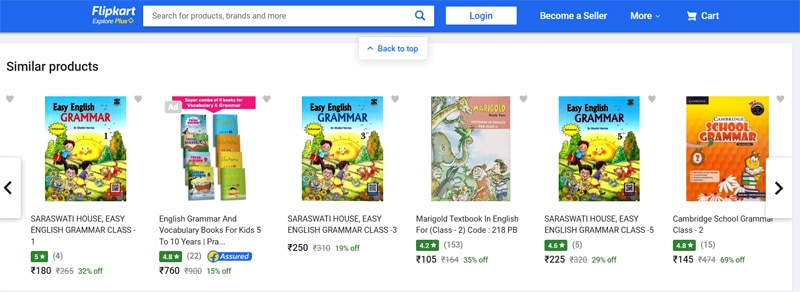
• Alternative product recommendations: You’ve probably tried to buy something you wanted, only to find it wasn’t available. But it’s unlikely you left the website after that. Instead, you may come across something similar, which you may or may not purchase. Companies utilise a recommendation system to keep customers online by providing them with alternatives to the product they want.
• Related product recommendations: Another important application of recommender systems is related product recommendations. When customers make a purchase, it’s only natural to offer them something complementary. If a customer purchases a wrist watch, the system may suggest a wallet, which goes well with it.
• Real-time true personalisation: With every second of customer activity on e-commerce sites, recommender systems can provide product or content or lifestyle recommendations. They can serve as a shopping assistant, using all the information the customer gives to offer improved recommendations, thus creating a better shopping experience.

Recommender systems: A broad categorisation

Content-based filters

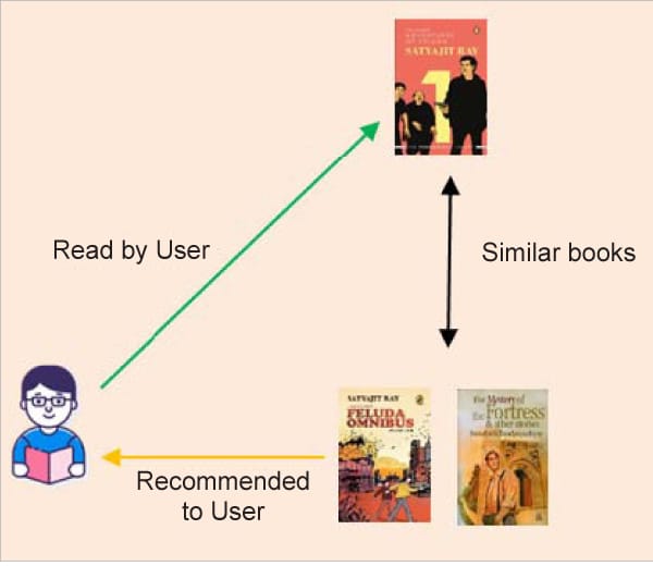
Content-based recommender systems give recommendations based on objects or user metadata. The user’s previous purchases are scrutinised. For example, if a user has previously read a book by a particular author or purchased a product from a particular brand, it is considered that the user has a preference for that author or brand and is likely to purchase a similar product in the future. For example, if a user likes the book ‘The Adventures of Feluda’ by Satyajit Ray, then the system recommends more books by the same author or other detective books like ‘The Mystery of the Fortress & Other Stories’.

Two types of data are used in this filtering. The first includes the user’s preferences, interests, and personal information such as age or, in some cases, the user’s history. The user vector represents this information. The second is an item vector, which is a collection of information about a product. The item vector contains all the information that can be used to calculate the similarity between things. Cosine similarity is used to determine the recommendations.

Collaborative filtering

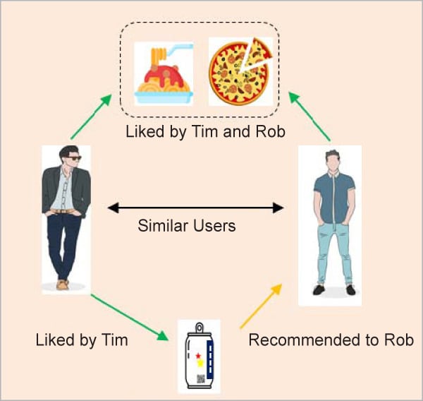
This is regarded as one of the most intelligent recommender systems, and is based on the similarity between different users and things such as e-commerce websites and online movie websites. It makes recommendations based on the preferences of comparable users. Similarity is not limited to the user’s preference; it can also be considered between distinct objects. If we have a big amount of knowledge about people and things, the algorithm will make more efficient recommendations.

Collaborative filtering is a method of recommending items that a user might enjoy based on the reactions of other users. It works by sifting through a huge group of people to locate a smaller group of users with likes similar to a specific user. It analyses their favourite things and creates a ranked list of recommendations.

A collaborative filtering system’s workflow is usually as follows:

• A user expresses his or her choices by rating system objects (for example, music, books, or movies). These ratings might be considered as an approximation of the user’s interest in the topic.
• The system matches this user’s preferences against other user preferences and finds the people with the most ‘similar’ choice.
• The system recommends items that similar users have rated the most but have not yet been rated by this user (the absence of rating is often considered as unfamiliarity with an item).

The main challenge of collaborative filtering is combining and weighing the preferences of user neighbours. Users can sometimes rate the recommended items right away. As aresult, over time, the system obtains a more accurate depiction of consumer preferences.

The math behind finding the ‘similarity’ to recommend

So, how does a recommender system determine ‘similarity’? The distance metric is used to do this. Similarity is a subjective concept that varies greatly depending on the domain and application. The points closest to each other are the most similar, while the points furthest apart are the least relevant. Two films, for example, may be comparable in terms of genre, length, or actors. When measuring distance between unrelated dimensions/features, caution is advised. The relative values of each element must be normalised, else the distance calculation will be dominated by one feature.

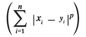
Minkowski distance: The Minkowski distance is the general form when the dimension of a data point is numeric. It’s a metric for vector spaces with real values. Minkowski distance can only be calculated in a normed vector space, which is a space where distances can be represented as a vector with a length that cannot be negative. Manhattan(r=1) and Euclidean(r=2) distance measurements are generalisations of this generic distance metric.

The formula shown above for Minkowski distance is in a generalised form, and we can manipulate it to get different distance metrics. Here, the ‘p’ value can be manipulated to give us different distances like:

• p = 1; when p is set to 1, it is Manhattan distance
• p = 2; when p is set to 2, it is Euclidean distance

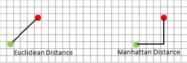
Manhattan distance: This distance is also known as taxicab distance or city block distance because of how it is calculated. The sum of the absolute differences of two places’ Cartesian coordinates is the distance between them – it’s the distance between two places when measured at right angles along axes. The formula is:

Euclidean distance: The square root of the sum of squares of the difference between the coordinates is given by the Pythagorean theorem:

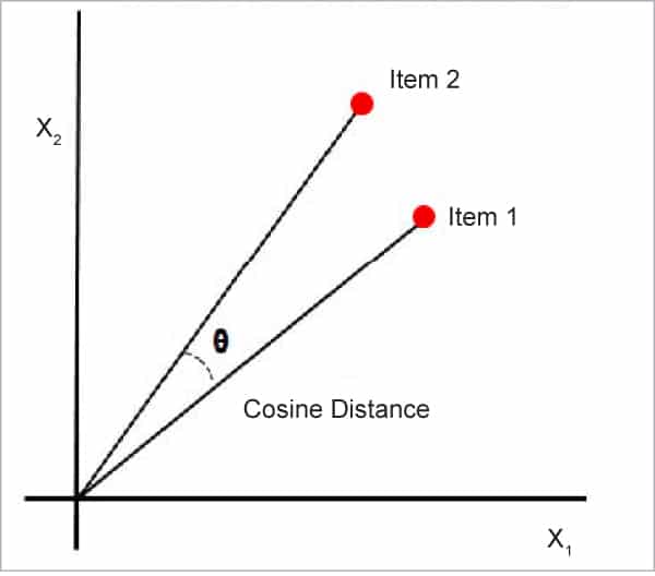
Cosine similarity: This is a metric that is useful in determining how similar the data objects are, irrespective of their size. Cosine similarity calculates the cosine of the angle between two vectors to determine how similar they are. In cosine similarity, data objects in a data set are treated as a vector. The formula to find the cosine similarity between two vectors is:

Cos(x, y) = x . y / ||x|| * ||y||

where,

• x, y = product (dot) of the vectors ‘x’ and ‘y’
• ||x|| and ||y|| = length of the two vectors ‘x’ and ‘y’
• ||x|| * ||y|| = cross product of the two vectors ‘x’ and ‘y’

The cosine similarity between two vectors is measured in ‘θ’. If θ = 0°, the ‘x’ and ‘y’ vectors overlap, thus proving they are similar. If θ = 90°, the ‘x’ and ‘y’ vectors are dissimilar.

Word embedding in the context of building a recommender system

Word embeddings are texts that have been translated into numbers, and there may be multiple numerical representations of the same text. But before we get into the specifics of word embedding, we need to consider the following question: Why do we need it?

Many machine learning algorithms and almost all deep learning architectures are unable to interpret strings or plain text in their raw form, as we all know. They need numbers as inputs to accomplish any task, including classification, regression, and so forth. Word embedding is nothing but the process of converting text data to numerical vectors. These vectors are then utilised to create a variety of machine learning models. In a sense, we could describe this as extracting features from text in order to create numerous natural language processing models.

We can transform text data into numerical vectors in a variety of ways. We’ll learn about numerous word embedding strategies with examples in this post, as well as how to apply them in Python.

Techniques for word embedding

The common and easy word embedding methods for extracting characteristics from text are:

• TF-IDF
• Bag of words
• Word2vec

TF-IDF

A popular word embedding technique for extracting features from corpus or language is TF-IDF. It is a statistical way of finding how important a word is to a document over other documents.

TF stands for ‘term frequency’. In TF, we assign a score to each word or symbol according to how frequently it appears. The frequency of a word is determined by the document’s length. This means that a word appears more frequently in huge documents than in small or medium documents. To solve this problem, we can normalise the frequency of a word by dividing it by the length of the document (total number of words).

Using this method, we may create a sparse matrix with the frequency of each word.

TF=Number of times a term occurs in a document/total number of words in a document

IDF

The full form of IDF is ‘inverse document frequency’. Here, we are assigning a score value to a word, which explains how infrequent a word is across all documents. Infrequent words have higher IDF scores.

IDF = log base e (total number of documents/number of documents that have the term)

TF - IDF = TF * IDF

TF-IDF value is increased based on the frequency of the word in a document. This approach is mostly used for document/text classification, and also successfully used by search engines like Google as a ranking factor for content.

When compared to the words that are relevant to a document, some common words (like ‘a’, ‘the’, ‘is’) appear relatively frequently in a huge text corpus. These popular words convey very little information about the document’s actual contents. If we fed the count data of these commonly occurring words directly to a classifier, the frequencies of rarer but more intriguing phrases would be overshadowed. So, ideally, what we want is to give lesser weightage to the common words occurring in almost all documents and give more importance to words that appear in a subset of documents.

The TF-IDF transform is frequently used to re-weigh count features into floating point values suitable for use by a classifier. This technique considers the occurrence of a word over the entire corpus, not just in a single document. Consider a business article — it will have more business-related terms like stock markets, prices, shares, and so on, than any other article, but terms like ‘a’, ‘an’, and ‘the’ will also appear frequently in it. As a result, this technique will punish certain high-frequency words.

Consider the table given below, which shows the total number of terms (tokens/words) in two papers.

Document 1		Document 2
TERM	COUNT	TERM	COUNT
this	1	this	1
is	1	is	2
about	2	about	1
pandemic	4	technology	1

Let’s define a few terminologies associated with TF-IDF now.

Term Frequency (TF) = (Number of times term t appears in a document)/(Number of terms in the document)
So, TF (This, Document1) = 1/8
TF (This, Document2) =1/5

This denotes the word’s contribution to the document, i.e., terms that are relevant to the document should appear frequently. For example, a document discussing a pandemic should use the word ‘pandemic’ frequently.

IDF = log (N/n), where, N is the number of documents and n is the number of documents a term t has appeared in.
So, IDF (This) = log (2/2) = 0.

So, what’s the best way to explain why IDF exists. Ideally, if a term appears multiple times in a paper, it is unlikely that it is significant to that document. However, if it appears in a subset of papers, it is likely that the word is relevant to the documents in which it appears.

Let us compute IDF for the word ‘pandemic’:

IDF (pandemic) = log (2/1) = 0.301.

Now, let us compare the TF-IDF for a common word ‘this’ and a word ‘pandemic’ which seems to be of relevance to Document 1.

TF-IDF (this, Document1) = (1/8) * (0) = 0
TF-IDF (this, Document2) = (1/5) * (0) = 0
TF-IDF (pandemic, Document1) = (4/8)*0.301 = 0.15

As you can see, for Document 1, the TF-IDF method heavily penalises the word ‘this’, but assigns greater weight to ‘pandemic‘. So, this may be understood as ‘pandemic’ is an important word for Document 1 from the context of the entire corpus.

Bag of words

Humans can understand a language in a fraction of a second. Machines, on the other hand, are unable to comprehend a language. We need to translate the text into a numerical format that the system can interpret. Because most machine learning and statistical models deal with quantitative data, we must transform all the texts to numbers. Bag of words is one of the simplest techniques to do this. In this approach, we perform two operations:

• Tokenization
• Vectors creation

Tokenization: This is the process of breaking down each sentence into words or smaller chunks. Each word or symbol is referred to as a token in this context. We can take unique words from the corpus after tokenization. The tokens we have from all the documents we’re examining for the bag of words construction are referred to as ‘corpus’.

Vectors creation: Here, the size of the vector is equal to the number of unique words of the corpus. We can fill each position of a vector with the corresponding word frequency in each sentence. Let’s look at an example.

• I like to drink tea.
• Tea is good for your health.
• Tea is more popular than coffee in India.

If we want to analyse the above sentences or build any ML model, we first need to convert them into numbers, as I mentioned above.

The first step is to tokenize the sentences. This is nothing but splitting the above three sentences into individual words.

The next step is to find all the unique words from the above sentences and build the vocabulary. We’ll have to make a dictionary with keys and values. The words in our corpus serve as keys, and the frequency of those terms throughout the corpus serves as values. To put it another way, simply count the number of times each word appears in each sentence.
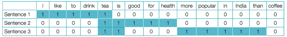
From Table 1, we can see the numbers corresponding to the respective sentences. The first row represents the vector for sentence 1. Given below are the vectors for:

Sentence 1 = [1,1,1,1,1,0,0,0,0,0,0,0,0,0,0]
Sentence 2 = [0,0,0,0,1,1,1,1,1,0,0,0,0,0,0]
Sentence 3 = [0,0,0,0,1,1,0,0,0,1,1,1,1,1,0]

The bag of words paradigm is based on this concept. The above vector representation can be used as an input for ML or statistical models.

Word2vec

In a sentence, every word is dependent on another word or words. Word dependencies must be captured if we are to uncover commonalities and relationships between words.

We can’t capture the meaning or relationship of words from vectors using the bag of words and TF-IDF approaches. Word2vec creates embeddings, which are vectors. The word2vec model takes a big corpus as input and outputs it in vector space. The dimensionality of this vector space could be in the hundreds. This vector space will be used to position each word vector.

In vector space, all words in a corpus that are closer to each other share a common context. In this space, a word vector contains the positions of associated words.

Continuous bag of words (CBOW) and skip-gram are two neural network-based versions offered by word2vec. The neural network model in CBOW takes a variety of words as input and predicts a target word that is closely connected to the input words’ context. The skip-gram design, on the other hand, takes one word as input and anticipates its closely related context terms.

CBOW is faster and finds better numerical representations for common words, although skip-gram can represent rare words effectively. Word2vec models excel at capturing semantic connections between words. Consider the relationship between a country and its capital, such as France’s capital, Paris, and Germany’s capital, Berlin. These models are best at doing semantic analysis, which is useful for making recommendations.

Applicability of word2vec models in building product recommendations: Word2vec uses the sequential nature of the text as a fundamental property of a natural language to produce vector representations of text. There is a word sequence in every sentence or phrase. We would have great difficulty understanding the text without this sequence.

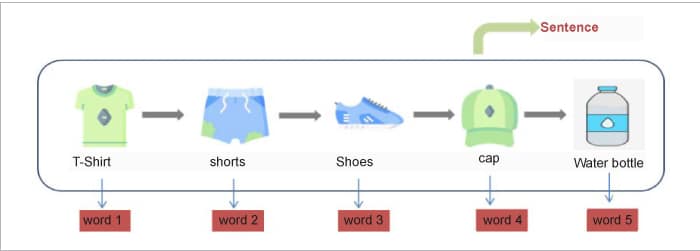
One such example is the purchases made by consumers on e-commerce websites online. There is generally a pattern in the buying behaviour of consumers. For instance, a person involved in sports-related activities might have an online buying pattern similar to what is shown in Figure 8.

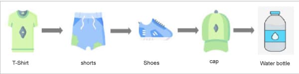
We can quickly locate related products if we can represent each of these things as a vector. So, if a user is looking at a product online, we can quickly offer related things to him or her based on the product’s vector similarity score. However, how can we obtain a vector representation of these items? Is it possible to obtain these vectors using the word2vec model? Yes, it is! Consider a customer’s purchasing history as a sentence, with the products as the words, as shown in Figure 9.

So we have seen how a recommender system works and the mathematics behind it. We have also covered some basics of the ML being used in such a system. In the next part of this two-part series of articles, we will see how we can apply the knowledge learnt here to build a recommender system in Python.