


In this fourteenth article in the R series, we shall explore the common probability distribution functions available in R.
We will use version 4.2.1 installed on Parabola GNU/Linux-libre (x86-64) for the code snippets.
$ R --version

R version 4.2.1 (2022-06-23) -- “Funny-Looking Kid”
Copyright (C) 2022 The R Foundation for Statistical Computing
Platform: x86_64-pc-linux-gnu (64-bit)

R is free software and comes with ABSOLUTELY NO WARRANTY.
You are welcome to redistribute it under the terms of the
GNU General Public License versions 2 or 3.
For more information about these matters see
https://www.gnu.org/licenses/.
Consider the mtcars data set in the lattice library:
> head(mtcars)
mpg cyl disp hp drat wt qsec vs am gear carb
Mazda RX4 21.0 6 160 110 3.90 2.620 16.46 0 1 4 4
Mazda RX4 Wag 21.0 6 160 110 3.90 2.875 17.02 0 1 4 4
Datsun 710 22.8 4 108 93 3.85 2.320 18.61 1 1 4 1
Hornet 4 Drive 21.4 6 258 110 3.08 3.215 19.44 1 0 3 1
Hornet Sportabout 18.7 8 360 175 3.15 3.440 17.02 0 0 3 2
Valiant 18.1 6 225 105 2.76 3.460 20.22 1 0 3 1
The summary() function can be used to produce the basic statistics of the data, as shown below:
> summary(mtcars)
mpg cyl disp hp
Min. :10.40 Min. :4.000 Min. : 71.1 Min. : 52.0
1st Qu.:15.43 1st Qu.:4.000 1st Qu.:120.8 1st Qu.: 96.5
Median :19.20 Median :6.000 Median :196.3 Median :123.0
Mean :20.09 Mean :6.188 Mean :230.7 Mean :146.7
3rd Qu.:22.80 3rd Qu.:8.000 3rd Qu.:326.0 3rd Qu.:180.0
Max. :33.90 Max. :8.000 Max. :472.0 Max. :335.0
The Tukey’s five number summary (minimum, lower-hinge, median, upper-hinge, and maximum) can be obtained using the fivenum() function, as follows:
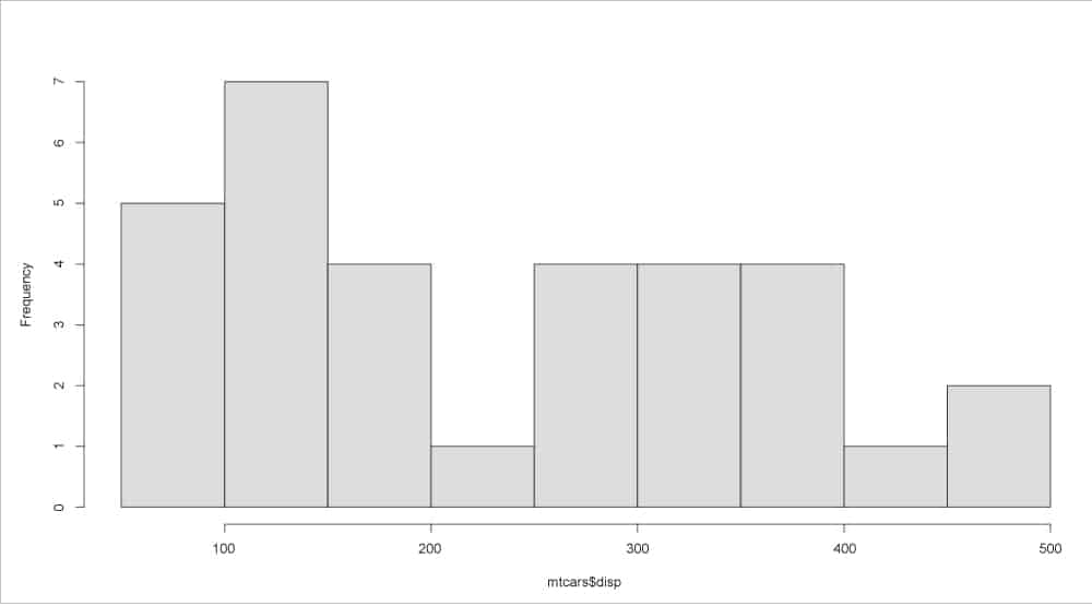
> mtcars$disp
[1] 160.0 160.0 108.0 258.0 360.0 225.0 360.0 146.7 140.8 167.6 167.6 275.8
[13] 275.8 275.8 472.0 460.0 440.0 78.7 75.7 71.1 120.1 318.0 304.0 350.0
[25] 400.0 79.0 120.3 95.1 351.0 145.0 301.0 121.0

> fivenum(mtcars$disp)
[1] 71.10 120.65 196.30 334.00 472.00
A histogram of the mtcars displacement data is shown in Figure 1.
The stem() function can generate a stem-and-leaf plot for input data. For example, we can obtain a plot for the mtcars cylinder, as demonstrated below:
> mtcars$cyl
[1] 6 6 4 6 8 6 8 4 4 6 6 8 8 8 8 8 8 4 4 4 4 8 8 8 8 4 4 4 8 6 8 4

> stem(mtcars$cyl)

The decimal point is at the |

4 | 00000000000
4 |
5 |
5 |
6 | 0000000
6 |
7 |
7 |
8 | 00000000000000
Uniform
The Uniform distribution has the following density function:
f(x) = 1/b-a
…where a <= x <= b. The runif() function generates random deviates, while the dunif() function gives the density, as illustrated below:
> d <- runif(10, min=0, max=1)
> d
[1] 0.48730291 0.26676446 0.15025110 0.77975962 0.42828890 0.05255129
[7] 0.54070173 0.54715839 0.42703064 0.31628728

> dunif(d)
[1] 1 1 1 1 1 1 1 1 1 1
These functions accept the following common arguments:
| Arguments | Description |
| x, q | A vector of quantiles |
| p | A vector of probabilities |
| n | Number of observations |
| log, log.p | A TRUE logical value indicates probabilities as log(p) |
| lower.tail | A TRUE logical value that probabilities are P[X <= x]] |
The specific set of arguments for the uniform distribution is given below:
| Arguments | Description |
| min, max | Finite lower and upper distribution limits |
Binomial
The density of the binomial distribution with probability ‘p’ and size ‘n’ is given by:
p(x) = select(n,x) p^x (1-p)^(n-x)
…where ‘x’ varies from 0 to n. The p(x) is calculated using the Loader’s algorithm. The pbinom() function gives the distribution function while the rbinom() function provides random values, as shown below:
> rbinom(5, 5, 1)
[1] 5 5 5 5 5

> rbinom(5, 5, 0.5)
[1] 3 2 2 4 2

> rbinom(5, 5, 0.25)
[1] 0 3 0 2 2
An example of pbinom() function for five successes in 10 trials, each having probability 0.5, is as follows:
> pbinom(5, 10, 0.5)
[1] 0.6230469
In addition to the common arguments listed previously, the binomial distribution function accepts the following arguments:
| Arguments | Description |
| size | Number of trials |
| prob | Probability of success in each trial |
Exponential
The exponential function for a given rate ‘lambda’ is given by:
f(x) = lambda {e}^{- lambda x}
…where x >= 0. The rexp() function provides random deviations, the qexp() function gives the quantile function, and the pexp() function provides the distribution function. A couple of examples are given below:
> rexp(5, rate = 1)
[1] 0.44090566 0.18508747 1.18596321 0.86235515 0.05020871

> pexp(d, rate = 1)
[1] 0.38571907 0.23414656 0.13950812 0.54148378 0.34837687 0.05119434
[7] 0.41766053 0.42140839 0.34755644 0.27114996
The specific ‘rate’ argument is applicable to the exponential function.
| Arguments | Description |
| rate | A vector of rates |
Geometric
The geometric distribution density with probability ‘p’ is defined as follows:
p(x) = p (1-p)^x
…where x = 0, 1, 2, etc, and ‘p’ is between 0 and 1. The rgeom() function for 10 observations and probability 0.5 is given below:
> d <- rgeom(10, 0.5)
> d
[1] 0 1 1 0 0 0 0 0 1 1
The pgeom() and qgeom() functions are based on closed-form formulae and provide the distribution and quantile functions, respectively.
> pgeom(d, 0.5)
[1] 0.50 0.75 0.75 0.50 0.50 0.50 0.50 0.50 0.75 0.75

> qgeom((1:10)/15, prob = 0.2)
[1] 0 0 0 1 1 2 2 3 4 4
The argument specific to the geometric function is given below:
| Arguments | Description |
| prob | Probability of success in each trial |
Normal
The normal distribution for mean ‘mu’ and standard deviation ‘sigma’ is given by:
f(x) = 1/(sqrt(2 pi) sigma) e^-((x - mu)^2/(2 sigma^2))
A sample of ten random values for mean 0 with standard deviation 1 can be generated using the rnorm() function, as follows:
> d <- rnorm(10, mean=0, sd=1)
> d
[1] 0.66512403 -0.43102217 0.50305386 1.55028087 1.20598557 0.33704698
[7] 0.09200192 0.67090448 -0.24424568 -0.78798191
Example uses of pnorm() and dnorm() functions are given below:
> pnorm (d, mean=0, sd=1)to
[1] 0.7470144 0.3332261 0.6925368 0.9394629 0.8860885 0.6319593 0.5366517
[8] 0.7488593 0.4035203 0.2153536

> dnorm(d, mean=0, sd=1)
[1] 0.3197763 0.3635536 0.3515265 0.1199568 0.1927928 0.3769138 0.3972575
[8] 0.3185439 0.3872184 0.2924691
The normal distribution specific arguments are listed for your reference below.
| Arguments | Description |
| mean | A vector of means |
| sd | A vector of standard deviations |
Poisson
The Poisson distribution density is defined as follows:
p(x) = lambda^x exp(-lambda)/x!
…where x = 0, 1, 2, … The mean and variance is lambda.
> d <- rpois(10, 0.9)
> d
[1] 2 2 1 3 1 2 1 1 0 0
The dpois() function gives the log density while the ppois() function gives the log distribution function. A couple of examples are given below:
> dpois(d, 0.9)
[1] 0.16466071 0.16466071 0.36591269 0.04939821 0.36591269 0.16466071
[7] 0.36591269 0.36591269 0.40656966 0.40656966

> ppois(d, 0.9)
[1] 0.9371431 0.9371431 0.7724824 0.9865413 0.7724824 0.9371431 0.7724824
[8] 0.7724824 0.4065697 0.4065697
The Poisson distribution function specific parameter is lambda, as shown below.
| Arguments | Description |
| lambda | A vector of non-negative means |
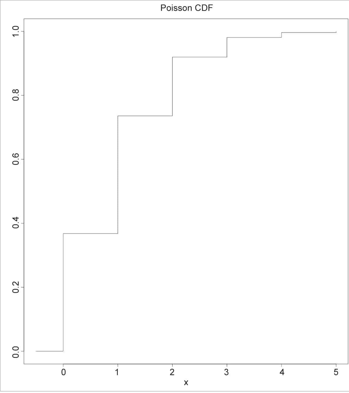
The Poisson CDF can be plotted in a graph, as shown below:
> x <- seq(-0.5, 5, 0.05)

> head(x)
[1] -0.50 -0.45 -0.40 -0.35 -0.30 -0.25

> plot(x, ppois(x, 1), type = “s”, ylab = “F(x)”, main = “Poisson CDF”)
Weibull
The shape parameter ‘a’ and scale parameter ‘b’ define the Weibull distribution density, as follows:
f(x) = (a/b) (x/b)^(a-1) exp(- (x/b)^a)
…where x > 0. The dweibull() function gives the density while the rweibull() function generates random deviates, as illustrated below:
> x <- c(0, rlnorm(10))
> x
[1] 0.0000000 0.5194988 2.2301132 0.1844523 0.5267321 0.5487738 1.3437871
[8] 2.0694222 3.6199835 6.3532987 5.9563711

> all.equal(dweibull(x, shape=1), dexp(x))
[1] TRUE

> rweibull(10, 5, 1)
[1] 0.5197291 0.6851027 1.0279023 1.1397738 0.8810083 0.7945575 0.5939060
[8] 0.8762381 0.7979457 0.6977511
The specific parameters for the Weibull distribution are as follows.
| Arguments | Description |
| shape, scale | shape and scale parameters |
You are encouraged to read the manual pages for the above R functions to learn more on their arguments, options and usage.


