























































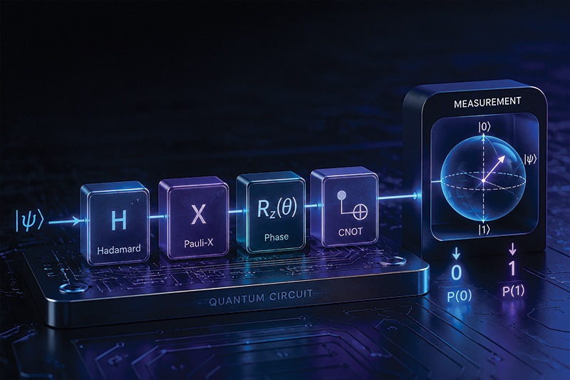

In the first article in this series on quantum computing (published in the May 2026 issue of OSFY), we explored some of the fundamental concepts of quantum computing, including qubits and the operation of the Hadamard gate. In this second article in the series, we will examine a few additional quantum gates and learn how measurements are performed on qubits to extract information from a quantum system.
As discussed in the previous article, our exploration of quantum computing will take place at three levels: the coding level, the mathematical level, and the hardware level. While we plan to use several platforms and programming languages to develop quantum algorithms throughout this series, we will begin with Qiskit, IBM’s quantum software development kit (SDK). In the previous article, we installed Qiskit and successfully executed our first quantum program.
Another theme we will explore throughout this series is the history of quantum computing and the latest developments in the field. In the previous article, we discussed the motivation behind quantum computers and the two groundbreaking algorithms that paved the way for practical quantum computing: Shor’s algorithm and Grover’s algorithm. In this article, we turn our attention to the various hardware architectures that have been proposed, tested, and developed in the quest to build a practical quantum computer.
Today, there are several competing approaches to building quantum computers, and it is still unclear which architecture will ultimately lead to large scale, fault-tolerant quantum computers. Some of the leading approaches include superconducting qubits, trapped-ion quantum computers, neutral-atom quantum computers, photonic quantum computers, etc. At present, no one can say with certainty which of these architectures will eventually dominate.
The situation bears some resemblance to the early days of classical computing. In the late 1940s and early 1950s, nobody knew whether the newly invented transistor would eventually replace vacuum tubes. Early transistors were expensive, relatively immature, and offered limited performance, while vacuum tubes had decades of engineering experience behind them and formed the basis of virtually all electronic computers of the time. Nevertheless, continuous improvements in semiconductor technology gradually tipped the balance in favour of transistors. By the 1960s, transistor-based computers had clearly emerged as the dominant technology, laying the foundation for the integrated circuits and modern microprocessors that power today’s digital world. History suggests that the eventual winner among competing quantum architectures may likewise be difficult to predict, and the technology that ultimately defines the quantum age may not necessarily be the one that appears most promising today.
Now, let us look at some of the major competing quantum computing architectures. The ordering below roughly follows what I personally consider to be their present level of practicality and maturity, beginning with the most widely used and commercially successful approaches and ending with those that remain highly speculative. It should be emphasised that this ranking reflects a personal opinion informed by the general consensus within the quantum computing community and is by no means universally accepted. The eventual winner may well turn out to be very different from what many researchers expect today.
Please keep in mind that, in each of the quantum computing architectures listed below, the fundamental hardware problem being addressed is the physical realisation of qubits—that is, how qubits are formed, manipulated, and protected from errors.
- Superconducting qubits operate at temperatures of around 15 millikelvin, colder than outer space. This is currently the most mature and commercially successful approach, pursued by IBM, Google, Rigetti, and IQM.
- Trapped-ion qubits use actual atoms, such as ytterbium or barium ions, suspended and manipulated using electromagnetic fields and laser pulses. Major players include IonQ, Quantinuum, and Alpine Quantum Technologies.
- Photonic qubits use photons as carriers of quantum information and are among the few architectures that can operate at room temperature. Companies developing this technology include PsiQuantum, Xanadu, and ORCA Computing
- Neutral-atom qubits employ individual atoms trapped by optical tweezers and can be arranged into arbitrary two-dimensional and even three-dimensional patterns. Important companies in this area include QuEra Computing, Atom Computing, and Pasqal.
- Silicon spin qubits encode information in the spins of electrons confined in silicon and can potentially leverage existing semiconductor manufacturing processes. Significant efforts are underway at Intel, Diraq, and several academic laboratories.
- Topological qubits are theoretically expected to be much more resistant to errors than other qubit technologies, but many of the required physical phenomena remain to be conclusively demonstrated. This approach is being pursued primarily by Microsoft and various research groups.
At present, no one can say with confidence which of these architectures will ultimately lead to large-scale, fault-tolerant quantum computers. History teaches us that technological winners are often difficult to predict.
Measurement in quantum computing
Now, let us do some quantum programming. First, let us modify the quantum program we wrote in the previous article and observe the changes when it is executed. The modified Python program, titled ‘qiskit2.py’ (with line numbers included for clarity), creates a single qubit and applies a Hadamard gate to it. However, unlike the previous version, this program also measures the state of the qubit.
1. from qiskit import QuantumCircuit

2. qc = QuantumCircuit(1, 1)

3. qc.h(0)

4. qc.measure(0,0)

5. print(qc.draw())
Now let us try to understand how this program works. Compared to the program ‘qiskit1.py’ discussed in the previous article, Line 2 has been modified and Line 4 has been newly added.
Line 2 creates a quantum circuit containing one qubit and one classical bit. The first argument, 1, specifies the number of qubits in the circuit, while the second argument, also 1, specifies the number of classical bits available for storing measurement results. As before, the qubit is initialised in the state |0by default. Line 4 performs a measurement operation on qubit 0 and stores the result in classical bit 0. The first argument, 0, denotes the qubit being measured, and the second argument, 0, denotes the classical bit in which the measurement outcome is recorded. After the measurement, the value stored in the classical bit will be either 0 or 1, depending on the outcome of the quantum measurement.
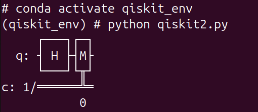
Recall that we installed Qiskit in a virtual environment named qiskit_env, which can be activated using the command ‘conda activate qiskit_env’. When the program ‘qiskit2.py’ is executed with the command ‘python qiskit2.py’, the output shown in Figure 1 is obtained. The output shows a visual representation of the quantum circuit generated by the program ‘qiskit2.py’. Compare this output with the one produced by ‘qiskit1.py’, the program discussed in the previous article.
Now, let us examine a quantum program that demonstrates the effect of a Hadamard gate on a qubit through measurement. Consider the program, titled ‘qiskit3.py’ (with line numbers included for clarity), shown below. This program applies a Hadamard gate to a qubit and then measures its state to illustrate the outcome of the operation.
1. from qiskit import QuantumCircuit

2. from qiskit_aer import AerSimulator

3. qc = QuantumCircuit(1, 1)

4. qc.h(0)

5. qc.measure(0, 0)

6. sim = AerSimulator( )

7. result = sim.run(qc, shots=1000). result( )

8. counts = result.get_counts( )

9. print(counts)
Now let us understand how the program works. Lines 1, 3, 4, and 5 are identical to those in ‘qiskit2.py’ and therefore require no further explanation. Line 2 imports the class AerSimulator from the package qiskit_aer. The AerSimulator enables us to execute quantum circuits on a classical computer and observe their measurement outcomes. Before proceeding, ensure that the AerSimulator has been installed. If you have not already done so, it can be installed using the command ‘pip install qiskit-aer’.
Line 6 creates an instance of the AerSimulator and assigns it to the variable sim. This simulator is then used to execute the quantum circuit. Line 7 runs the circuit on the simulator. The argument ‘shots=1000’ instructs the simulator to execute the circuit 1,000 times. A large number of shots is necessary because a single measurement reveals only one outcome—either 0 or 1. By repeating the experiment many times, we can estimate the probabilities associated with the possible outcomes. The method result( ) returns an object containing the results of all these executions. Line 8 extracts the measurement statistics from the result object and stores them in the variable counts. These statistics are returned as a dictionary in which the keys represent the measurement outcomes and the values indicate the number of times each outcome occurred. Line 9 displays the contents of the dictionary counts.
Since the qubit is in an equal superposition of |0 and |1, the outcomes 0 and 1 are expected to occur with approximately equal frequency. However, the counts will generally not be exactly equal because quantum measurement is inherently probabilistic. Unlike the previous examples, we will execute ‘qiskit3.py’ multiple times to observe the probabilistic nature of quantum computing. Figure 2 shows the results of five successive executions of the program.
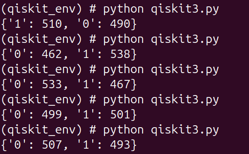
Now, let us examine the output obtained from five successive executions of the program ‘qiskit3.py’. Recall that the Hadamard gate places the qubit in the state |ψ=√(1/2)(|0+|1) which implies that the probabilities of obtaining the outcomes 0 and 1 upon measurement are both 50%. Since the circuit is executed 1000 times (1000 shots), one might be tempted to expect exactly 500 occurrences of 0 and 500 occurrences of 1. However, quantum measurement is inherently probabilistic, and each measurement outcome is random. Consequently, the actual numbers fluctuate from one execution of the program to another, giving results such as 510–490, 462–538, or 499–501. These deviations are perfectly normal and are analogous to the outcome of tossing a fair coin 1000 times, where one rarely obtains exactly 500 heads and 500 tails. As the number of shots increases, the measured frequencies tend to approach the theoretical probabilities predicted by quantum mechanics. It is important to note that these fluctuations are not caused by imperfections in the simulator. Rather, they are a manifestation of the intrinsic probabilistic nature of quantum measurement itself, one of the most fundamental features of quantum mechanics.
Now, let us try to understand how critical measurement is in quantum computing and how quantum mechanics plays a central role in the process. In a classical computer, reading a bit does not disturb its value. If a bit stores 0, reading it simply reveals 0 and the bit remains 0. Similarly, if the bit stores 1, reading it reveals 1 without changing the state of the bit.
A qubit behaves very differently. Consider the superposition state |ψ=√(1/2)(|0+|1). When this qubit is measured, the outcome is 0 with probability 1/2 and 1 with probability 1/2. More importantly, the act of measurement changes the state of the qubit itself. If the outcome is 0, the qubit collapses to the state |0; if the outcome is 1, it collapses to the state |1. This phenomenon, known as wavefunction collapse, is one of the most surprising features of quantum mechanics.
The collapse of the wavefunction is both a curse and a boon. It is a curse because measurement destroys the superposition and the original quantum state cannot be recovered. However, it is also a boon because measurement provides the classical information that constitutes the final output of a quantum computation. Thus, measurement acts as a bridge between the quantum world and the classical world.
Pauli Gates
As promised in the previous article, we shall continue our exploration of quantum gates in this article. Recall that there are a large number of quantum gates, and it is neither practical nor necessary to discuss all of them at once. Instead, we will gradually introduce more and more gates as the series progresses. We shall begin by familiarising ourselves with the various single-qubit quantum gates before moving on to multi-qubit gates, which form the building blocks of more sophisticated quantum algorithms.
In this article, we will expand our knowledge of quantum gates by studying the Pauli gates, named after Wolfgang Pauli, the brilliant Austrian theoretical physicist who was awarded the 1945 Nobel Prize in Physics. Once again, we encounter a Nobel laureate whose work has had a profound influence on quantum computing—a recurring theme in the history of this fascinating field.
There are three Pauli gates, namely the Pauli-X, Pauli-Y, and Pauli-Z gates. All three are single-qubit quantum gates and play a fundamental role in quantum computing. Let us begin by examining the Pauli-X gate and see how it is implemented in Qiskit. Consider the program ‘qiskit4.py’ (with line numbers included for clarity), shown below.
1. from qiskit import QuantumCircuit

2. from qiskit_aer import AerSimulator

3. qc = QuantumCircuit(1, 1)

4. qc.x(0)

5. qc.measure(0, 0)

6. sim = AerSimulator()

7. result = sim.run(qc, shots=1000). result()

8. counts = result.get_counts()

9. print(counts)
The program shown above is almost identical to ‘qiskit3.py’ discussed earlier. The only difference is in Line 4, where the Hadamard gate has been replaced by the Pauli-X gate. Line 4 applies the Pauli-X gate to qubit 0. Since a newly created qubit is initialised in the state |0, the action of the Pauli-X gate transforms it to the state |1. In this sense, the Pauli-X gate plays a role analogous to that of the classical NOT gate, which changes 0 to 1 and 1 to 0.
Before examining the output of the program ‘qiskit4.py’, let us modify it slightly by inserting another line of code ‘qc.x(0)’ (identical to Line 4), immediately after Line 4. The resulting program will be referred to as ‘mod_qiskit4.py’.
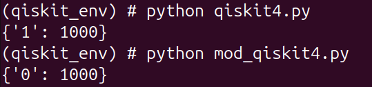
Figure 3 shows the outputs obtained from the programs ‘qiskit4.py’ and ‘mod_qiskit4.py’. In ‘qiskit4.py’, a single Pauli-X gate is applied to a qubit initially in the state |0. Consequently, the qubit is transformed to the state |1, and all 1000 measurements produce the outcome 1. In ‘mod_qiskit4.py’, the Pauli-X gate is applied twice in succession. The first application changes the state from |0 to |1, while the second application changes it back from |1 to |0. As a result, all 1000 measurements yield the outcome 0. Thus, applying the Pauli-X gate twice restores the original state of the qubit. This demonstrates an important property of the Pauli-X gate: it is reversible and acts as its own inverse. In other words, two successive applications of the Pauli-X gate are equivalent to performing no operation at all on the qubit. Notice the contrast with the Hadamard gate: here, the outcome is completely deterministic, with no randomness involved.
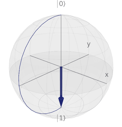
In the previous article in the series, we discussed the Bloch sphere and used it to visualise the effect of the Hadamard gate on a qubit. Let us now revisit the Bloch sphere to understand the action of the Pauli-X gate. Recall that the state |0 is represented by an arrow pointing towards the north pole of the Bloch sphere, while the state |1 corresponds to an arrow pointing towards the south pole. Figure 4 shows the effect of applying the Pauli-X gate to a qubit initially in the state |0. It can be seen that the state vector is rotated from the north pole to the south pole, thereby transforming the state |0 into |1. If the Pauli-X gate is applied once again, the state vector returns to the north pole, demonstrating that the Pauli-X gate is reversible and acts as its own inverse.
Let us now try to understand the mathematics behind the operation of the Pauli-X gate. Recall that, in vector form, the states |0 and |1 are represented by [1 0]ᵀ and [0 1]ᵀ, respectively. Notice the superscript T, which indicates that these are column vectors. In the previous article, we saw how the Hadamard gate is represented by a 2 × 2 matrix. Similarly, the Pauli-X gate is also represented by a 2 × 2 matrix. Figure 5 shows the matrix representation of the Pauli-X gate. The figure also illustrates how the Pauli-X matrix acts on the column vector corresponding to |0 and transforms it into the column vector corresponding to |1. It would be a worthwhile exercise to perform the same matrix multiplication on the column vector representing |1 and verify that the result is the column vector corresponding to |0. This confirms that the action of the Pauli-X gate on the computational basis states is analogous to that of the classical NOT gate, which interchanges 0 and 1.

The uniqueness of this series lies in its three-level approach to quantum computing. Throughout the series, we shall repeatedly encounter the same quantum operation from three complementary perspectives: the programmer’s perspective, the mathematician’s perspective, and the experimental physicist’s perspective. We have already seen how the Pauli-X gate is invoked at the coding level using Qiskit, and we have also examined the mathematical operation corresponding to the gate. It is now time to explore the hardware side of implementing the Pauli-X gate. At this point, however, we encounter a dilemma: which quantum computing architecture should we choose as our representative platform? After much deliberation, I have decided to focus on superconducting qubits, since the superconducting approach currently remains the most popular, commercially mature, and widely deployed quantum computing architecture in the world.
At the hardware level, a superconducting qubit is physically realised using a tiny superconducting circuit containing Josephson junctions and cooled to a temperature of about 15 millikelvin. The states |0 and |1 correspond to two distinct quantum energy levels of this circuit. When a Pauli-X gate is applied to a qubit initially in the state |0, the quantum processor generates a precisely calibrated microwave pulse whose frequency matches the energy difference between these two levels. This pulse causes the state vector of the qubit to rotate by 180° about the x-axis of the Bloch sphere, thereby transferring the qubit from the north pole to the south pole and changing its state from |0 to |1. Thus, what appears in Qiskit as the simple statement ‘qc.x(0)’ is, at the hardware level, realised by an exquisitely controlled electromagnetic pulse manipulating a quantum system cooled to temperatures colder than outer space.
The Pauli-X gate is perhaps the most intuitive of the three Pauli gates, since it has a direct classical analogue in the form of the classical NOT gate. The effects of the Pauli-Y and Pauli-Z gates are more subtle and require an understanding of one of the most important concepts in quantum computing: the phase of a quantum state. We shall therefore postpone a detailed discussion of these two gates until the next article in this series.
It is now time to wind up our discussion. In the next article, we will delve deeper into quantum programming and continue our exploration of quantum gates, uncovering how phase plays a crucial role in the behaviour of quantum systems.