

























































In this third article in the series on quantum computing, we will develop an intuitive understanding of the quantum phase and explore how it influences the behaviour of quantum systems.
In the second article in this series on quantum computing (OSFY, July 2026), we explored several competing hardware architectures for building quantum computers and examined how quantum measurement enables us to extract classical information from a quantum system. We concluded by studying the Pauli-X gate, perhaps the most intuitive of the three Pauli gates (Pauli-X, Pauli-Y, and Pauli-Z), owing to its close resemblance to the classical NOT gate. However, as we noted at the end of that article, the remaining two Pauli gates cannot be fully understood without first introducing one of the most fundamental—and often one of the most challenging—concepts in quantum computing: quantum phase.
By now, I assume that readers following this series have become familiar with several fundamental concepts of quantum computing, including qubits, superposition, quantum measurement, the Hadamard and Pauli-X gates, the Bloch sphere, the matrix representation of quantum states and gates, basic programming with Qiskit, and a brief overview of superconducting quantum hardware. These concepts provide the foundation for everything that follows.
However, we have only just begun our journey, and many important questions remain unanswered. Why are quantum computers powerful? Why is a single qubit not enough? Why does quantum phase matter? And what makes quantum algorithms fundamentally different from classical probabilistic algorithms? Don’t worry—we have just started flexing our muscles. In the coming articles, we will answer each of these questions
The defining feature of this series is its three-level approach to understanding quantum computing—examining every important concept from the perspectives of programming, mathematics, and hardware. This integrated approach is rarely found in introductory tutorials or textbooks, which often focus on only one of these aspects. Another promise of this series is to explore not only the technical foundations of quantum computing but also its history, current developments, future directions, and the many misconceptions that surround this fascinating field. So, before we move any further, let us begin by bursting two of the most common myths about quantum computing—myths that are widely repeated but fundamentally incorrect.
One of the most common myths about quantum computing is that a quantum computer can “try every possible answer simultaneously.” Although this sounds fascinating, it is not an accurate description of how quantum computers work. A qubit can indeed exist in a superposition of states, allowing a quantum system to represent many possibilities at once. However, when the qubits are measured, only one outcome is obtained—not all possible answers. If quantum computers could simply examine every possible solution and read out the correct one, many computationally difficult problems would become trivial, which is certainly not the case.
The real power of quantum computing lies not in trying every answer simultaneously, but in manipulating quantum states so that the correct answer becomes more likely to appear when the final measurement is made. How this happens is one of the central ideas in quantum computing, involving concepts such as quantum phase, interference, and multi-qubit systems.
The second myth is that quantum computers will replace classical computers. Quantum computers are not designed to replace the laptops, desktops, smartphones, or servers that we use every day. In fact, everyday tasks such as web browsing, word processing, video streaming, email, and gaming are performed far more efficiently by classical computers. For such applications, quantum computers offer little or no advantage.
Instead, quantum computers are expected to serve as highly specialised machines that complement rather than replace classical computers, much like GPUs today accelerate graphics processing and artificial intelligence. They are likely to excel at specific classes of problems, including quantum simulation, cryptography, optimization, and certain machine learning tasks, while conventional computers continue to handle most of the everyday computing. The future of computing is therefore unlikely to be a choice between classical and quantum computing. Rather, it will be a partnership in which classical and quantum computers work together, each solving the problems for which it is best suited.
Now, let us turn our attention to one of the most fundamental—and often one of the most challenging—concepts in quantum computing: quantum phase. To develop an intuitive understanding of this idea, we shall study the two remaining Pauli gates: Pauli-Y and Pauli-Z. Let us begin with the lesser of these two evils—the Pauli-Z gate. I jokingly refer to them as ‘evil’ because they are notoriously difficult to understand and typically require much more explanation than the Pauli-X gate. Fortunately, there is an excellent visual aid that makes these concepts far more intuitive. As in the previous two articles, we shall once again make use of the online Bloch sphere simulator available at https://bloch.kherb.io/. By observing how these gates rotate the state vector on the Bloch sphere, the role of quantum phase becomes much easier to appreciate.
Open the Bloch sphere simulator and, from the Quantum gates menu, click the Z button corresponding to the Pauli-Z gate. What did you observe? At first glance, it appears that nothing happened. The arrow still points towards the north pole of the Bloch sphere, just as it did before. Is something wrong with the simulator? Not at all. In fact, the simulator is behaving exactly as it should.
The Pauli-Z gate performs a 180° (π radians) rotation about the z-axis of the Bloch sphere. Since the qubit is initially in the state |0〉, its state vector already lies along the z-axis. Rotating an arrow about its own axis does not change its visible direction—just as spinning a perfectly straight pencil about its own length leaves it looking exactly the same. The rotation has indeed taken place, but it cannot be seen from the orientation of the arrow alone.
This hidden change is known as a phase change. Unlike a bit flip, which changes the observable state of a qubit, a phase change does not immediately alter what we see or what we obtain when we measure the qubit. Instead, it changes the relative phase of the quantum state. Although this phase is invisible by itself, it profoundly influences how the qubit behaves when subsequent quantum gates are applied. In other words, phase cannot be observed directly, but its effects become evident through later quantum operations. As we shall soon discover, this seemingly invisible property lies at the heart of quantum interference and many of the remarkable advantages offered by quantum computing. Now, let us execute three related Qiskit programs to explore the effect of the Pauli-Z gate.
The first program, ‘qiskit3.pyʼ, was introduced in the previous article. It applies a Hadamard gate to a qubit and then measures the qubit to demonstrate how the Hadamard gate creates an equal superposition of the |0〉 and |1〉 states.
Let us now examine a quantum program that demonstrates the effect of the Pauli-Z gate on a qubit. Consider the program ‘qiskit5.py’, shown below. Starting from the initial state |0〉, the program first applies a Hadamard gate to create an equal superposition of |0〉 and |1〉 . It then applies a Pauli-Z gate, followed by a measurement of the qubit. By comparing the output of this program with that of the previous one, we can investigate whether the Pauli-Z gate has any observable effect on the measurement outcome. Notice that the only new line of code requiring explanation is ‘qc.z(0)’, which applies a Pauli-Z gate to the single qubit in the circuit.
from qiskit import QuantumCircuit
from qiskit_aer import AerSimulator

qc = QuantumCircuit(1, 1)
qc.h(0)
qc.z(0)
qc.measure(0, 0)

sim = AerSimulator()

result = sim.run(qc, shots=1000).result()
counts = result.get_counts()
print(counts)
The program ‘qiskit6.pyʼ, shown below, extends ‘qiskit5.pyʼ by inserting a second Hadamard gate after the Pauli-Z gate and before measurement. We add this second Hadamard gate because it converts the otherwise hidden phase information into measurable probabilities, making the effect of the Pauli-Z gate observable. As we shall see, this seemingly minor modification dramatically changes the outcome of the computation.
from qiskit import QuantumCircuit
from qiskit_aer import AerSimulator

qc = QuantumCircuit(1, 1)
qc.h(0)
qc.z(0)
qc.h(0)
qc.measure(0, 0)

sim = AerSimulator()

result = sim.run(qc, shots=1000).result()
counts = result.get_counts()
print(counts)
Execute the three programs after activating the virtual environment qiskit_env, as described in the previous articles. Figure 1 shows the measurement results from these programs. What conclusions can we draw from these outputs.
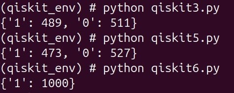
Observe that the outputs of ‘qiskit3.pyʼ and ‘qiskit5.pyʼ are nearly identical, with approximately equal numbers of 0s and 1s. This indicates that inserting a Pauli-Z gate before measurement does not alter the measurement probabilities. However, the output of ‘qiskit6.pyʼ is strikingly different. After applying the second Hadamard gate, the qubit is measured exclusively in the state |1〉. Clearly, the Pauli-Z gate was not “doing nothing” after all—it was modifying the phase of the quantum state, an effect that becomes observable only after a subsequent quantum operation. This simple experiment illustrates the essence of quantum interference: although the phase introduced by the Pauli-Z gate is invisible by itself, it changes how later quantum operations combine probability amplitudes.
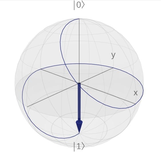
To verify this behaviour visually, let us return to the Bloch sphere simulator. Perform the same sequence of operations—Hadamard, Pauli-Z, and Hadamard (H–Z–H)—on the Bloch sphere. The final configuration is shown in Figure 2. Notice that the qubit ultimately points towards the south pole, corresponding to the state |1〉. perfectly matches the measurement results produced by the program ‘qiskit6.py’.
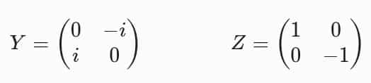
Let us now turn our attention to the mathematical representation of the Pauli-Y and Pauli-Z gates. As shown in Figure 3, both gates, like the Pauli-X gate, are represented by 2 × 2 matrices. Using the rules of matrix multiplication, verify that multiplying the Pauli-Z matrix by the column vector representing the state |0〉 leaves the state unchanged, while multiplying it by the column vector representing |1〉 introduces a minus sign, producing the state −|1〉. Similarly, verify that multiplying the Pauli-Y matrix by the column vector representing |0〉 yields i|1〉, whereas multiplying it by the column vector representing |1〉 gives −i|1〉
(Here, i denotes the imaginary unit, defined by the property i2 = −1.). These simple calculations reveal that, unlike the Pauli-X gate, the Pauli-Y and Pauli-Z gates not only affect the computational basis states but also introduce changes in their quantum phase.
What happens at the hardware level when a Pauli-Z gate is applied to a superconducting qubit? Unlike a Pauli-X gate, which is implemented by applying a resonant microwave pulse that physically drives the qubit between the |0〉 and |1〉 states, a Pauli-Z gate does not move the qubit from one state to the other. The qubit remains in the same energy level, while only the relative phase between |0〉 and |1〉 is modified. In most modern superconducting quantum processors, this operation is implemented as a virtual Z gate. Rather than sending an additional microwave pulse to the qubit, the control electronics simply update the phase reference of all subsequent microwave pulses by the required angle. Since no physical pulse is applied, the operation is effectively instantaneous, introduces virtually no additional decoherence, and contributes negligible gate error. As a result, the Pauli-Z gate is one of the fastest and highest-fidelity quantum operations available on today’s superconducting quantum computers.
Let us now turn our attention to the Pauli-Y gate, perhaps the most challenging of the three Pauli gates to understand. We have already seen its mathematical action through matrix multiplication, but what does the gate actually do? To build an intuitive understanding, let us temporarily sacrifice a little mathematical rigour. A useful way to think about the Pauli-Y gate is that it combines the effects of the Pauli-X and Pauli-Z gates. In other words, it performs both a bit flip and a phase flip simultaneously. Recall that the Pauli-X gate flips the qubit from |0〉 to |1〉 (and vice versa) by performing a 180° rotation about the x-axis of the Bloch sphere. The Pauli-Z gate, on the other hand, leaves the computational basis states unchanged but introduces a 180° phase shift by rotating the qubit about the z-axis. The Pauli-Y gate combines these two ideas into a single operation, corresponding to a 180° rotation about the y-axis of the Bloch sphere.
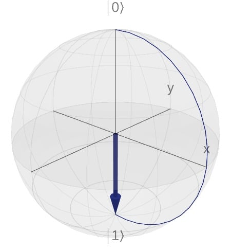
Now, let us observe the effect of the Pauli-Y gate on the Bloch sphere. Figure 4 shows the evolution of the qubit when the Pauli-Y gate is applied to the state |0〉. Notice that the final state is again |1〉, just as it was for the Pauli-X gate discussed in the previous article. However, the two gates reach this state by following entirely different paths on the Bloch sphere. The Pauli-X gate performs a 180° rotation about the x-axis, whereas the Pauli-Y gate performs a 180° rotation about the y-axis.
Does the path taken really matter? To build some intuition, let me use a simple analogy (assuming you are familiar with the geography of India). Suppose you and your friend are both travelling from Delhi to Chennai. Your flight goes via Kolkata, while your friend’s flight goes via Mumbai. By evening, when someone asks where the two of you are, the answer is the same—you have both reached Chennai. However, if someone asks at noon how far each of you is from Guwahati, the answers will be quite different. Although your destinations are identical, the routes you followed were not.
The Pauli-X and Pauli-Y gates behave in a similar manner. Starting from |0〉, both eventually reach |1〉, but the state vector follows a different trajectory on the Bloch sphere. For the basis states |0〉 and |1〉, this difference is not directly observable. However, for qubits in superposition states, the different rotations performed by the Pauli-X and Pauli-Y gates produce different relative phases, which can significantly influence the outcome of subsequent quantum operations. Understanding this subtle role of phase is one of the keys to understanding why quantum computing is fundamentally different from classical computing. As this is a challenging concept, we shall revisit it several times in the articles that follow in this series.
Now, let us examine the effect of the Pauli-Y gate on a superconducting qubit at the hardware level. Unlike the Pauli-X gate, which is implemented using a resonant microwave pulse that rotates the qubit by 180° about the x-axis, and the Pauli-Z gate, which is typically realized as a virtual Z gate by simply updating the phase reference of subsequent microwave pulses, the Pauli-Y gate requires both operations. In practice, it is implemented by applying a microwave pulse whose phase is shifted by 90° relative to that used for the Pauli-X gate, producing a 180° rotation about the y-axis of the Bloch sphere. Equivalently, the operation may be viewed as a suitable combination of Pauli-X and Pauli-Z operations. Consequently, the Pauli-Y gate performs both a bit flip and a phase flip simultaneously. Although its implementation is slightly more involved than that of the Pauli-X gate, it remains a high-fidelity operation on modern superconducting quantum processors.
Before concluding this article, let us briefly examine one of the most important hardware components in a superconducting quantum computer—the Josephson junction. In the previous article, we decided to focus most of our hardware discussions on superconducting qubits, since they currently represent the most mature and commercially successful quantum computing technology. However, as we also noted, no guarantee that superconducting qubits will ultimately emerge as the winning architecture among the many competing quantum technologies. Nevertheless, understanding the Josephson junction provides valuable insight into how today’s superconducting quantum processors, such as those developed by IBM and Google, actually work. It is no exaggeration to say that the Josephson junction is the heart of these quantum processors.
A Josephson junction consists of two superconducting materials separated by an extremely thin insulating layer, typically only a few nanometres thick. Although the insulating layer should, in principle, prevent electric current from flowing, quantum mechanics allows pairs of electrons, known as Cooper pairs, to tunnel through the barrier. This remarkable phenomenon, known as the Josephson effect, was predicted by the British physicist Brian D. Josephson in 1962 and later earned him the Nobel Prize in Physics. By the third article in this series, it has almost become a cliché to point out that the history of quantum computing is filled with Nobel laureates!
It is important to understand that programmers never interact with the Josephson junction directly. When we write a Qiskit statement such as qc.x(0) or qc.h(0), we are specifying a logical quantum operation rather than controlling the hardware itself. The quantum control system automatically translates these instructions into precisely calibrated microwave pulses, which manipulate the superconducting qubit through the Josephson junction. Thus, what appears as a single line of Qiskit code corresponds, at the hardware level, to an intricate sequence of physical processes occurring inside a quantum processor operating at temperatures of only a few millikelvin.
Although Qiskit focuses primarily on programming quantum circuits, there are specialised open source tools for modelling and designing superconducting quantum hardware. QuTiP (Quantum Toolbox in Python) is widely used to simulate the dynamics of quantum systems, including superconducting qubits and Josephson-junction-based circuits. Quantum Metal (formerly Qiskit Metal) is another open source framework that enables researchers to design and analyse superconducting quantum devices before they are fabricated. Although we will explore these tools in much greater detail later in this series, it is worthwhile to get a brief glimpse of QuTiP.
Consider the following sample program, which constructs the Hamiltonian of a simple two-level quantum system—the basic mathematical model used to describe a superconducting qubit.
from qutip import sigmax, sigmaz

omega = 5.0
delta = 1.0
H = 0.5 * omega * sigmaz() + 0.5 * delta * sigmax()
print(H)
The program above is not a complete physical simulation of a Josephson-junction circuit, but rather the simplest Hamiltonian that captures the behaviour of a superconducting qubit. More realistic Josephson-junction models involve additional physical parameters, non-linear circuit elements, and time-dependent microwave control pulses. We shall postpone these fascinating topics until a much later article in this series, where we will explore quantum hardware in greater depth using tools such as QuTiP and Quantum Metal.
So far our discussion has been confined to single-qubit systems. A lone qubit, fascinating though it is, cannot demonstrate the true power of quantum computing. That power begins to emerge only when multiple qubits interact with one another. In the next article, we will leave the world of isolated qubits behind and explore the CNOT gate, one of the most important quantum gates, which serves as the gateway to one of the strangest and most remarkable phenomena in modern physics—quantum entanglement, famously described by Albert Einstein as “spooky action at a distance.”