

























































We began this series with a simple question: why should someone already fluent in Python bother learning SageMath? Fourteen articles later, we have traversed graph theory, cybersecurity, cryptography, and the opening landscapes of number theory, and in doing so, I hope the answer has become self-evident. SageMath is not merely a mathematical dialect of Python; it is a fully equipped laboratory for scientific computing that reveals new capabilities the deeper one ventures into it. In this 15th and last article in the series, we shall explore a few more beautiful corners of that laboratory
In the previous article of this series (published in the April 2026 issue of OSFY), we began our exploration of number theory and examined several number-theoretic functions provided by SageMath. Throughout this series, we have seen that prime numbers occupy a central place in computer science, particularly in algorithms related to cryptography, cybersecurity, and computational number theory. Consequently, primality testing is one of the most fundamental operations performed by mathematical software. In the previous article, we explored several SageMath functions for primality testing and related computations. In this article, we will turn our attention to a few famous number-theoretic conjectures to appreciate the beauty and elegance of this branch of mathematics. Number theory is unique in that it contains centuries-old unsolved problems whose statements are so simple that they can be understood not only by professional mathematicians but even by high school students, yet they continue to challenge some of the greatest mathematical minds.
One of the oldest unsolved problems in number theory is the Goldbach Conjecture, proposed by the Prussian mathematician Christian Goldbach in 1742. It states that every even integer greater than 2 can be expressed as the sum of two prime numbers. For example, 10=3+7, 20=3+17, and 100=3+97. Although the conjecture has been verified computationally for extremely large numbers, no general mathematical proof has yet been discovered. Using SageMath, we can easily investigate the conjecture for any given even integer. The simple SageMath program goldbach48.sage, shown below, searches for a pair of prime numbers whose sum equals the given even integer and returns the first such pair that it finds. Notice that the program relies on just two built-in SageMath functions, prime_range( ) and is_prime( ). The function prime_range( ) efficiently generates prime numbers within a specified range, while is_prime( ) determines whether a given integer is prime. Both functions are highly optimized in SageMath, allowing the program to test the conjecture for very large integers much more efficiently than a straightforward implementation using basic Python code.
def goldbach(n):

for p in prime_range(2, n):

if is_prime(n - p):

return (p, n - p)

return None

print(goldbach(123456780))
Another famous unsolved problem in number theory is the Twin Prime Conjecture, first formally stated in the 19th century. It states that there exist infinitely many pairs of prime numbers that differ by two. Such pairs are known as twin primes. Examples include (3,5), (5,7), (11,13), and (41,43). Although twin prime pairs become increasingly rare as numbers grow larger, millions of such pairs have been discovered through extensive computer searches. However, no mathematical proof has yet established that infinitely many twin prime pairs exist. Using SageMath, we can easily search for twin prime pairs within any specified range and identify the largest twin prime pair found in that range. The simple SageMath program twinprime49.sage, shown below, searches for all twin prime pairs less than a specified limit and returns the largest pair found. Notice that the function is_prime( ) used in the program is a highly optimized primality-testing function provided by SageMath, enabling the program to efficiently search for twin prime pairs.
def largest_twin_prime(limit):
largest = None
for p in prime_range(2, limit):
if is_prime(p + 2):
largest = (p, p + 2)
return largest
limit = 1000000
pair = largest_twin_prime(limit)
print(pair)
Another famous unsolved problem in mathematics is the Collatz Conjecture, proposed by the German mathematician Lothar Collatz in 1937. The conjecture begins with any positive integer. If the number is even, divide it by 2; if it is odd, multiply it by 3 and add 1. Repeating this process generates a sequence of integers. The Collatz Conjecture states that every positive integer eventually reaches the value 1, regardless of the starting number. Despite its remarkably simple statement, no proof or counterexample has yet been discovered. For example, starting with 6 produces the sequence 6 → 3 → 10 → 5 → 16 → 8 → 4 → 2 → 1, while starting with 11 gives 11 → 34 → 17 → 52 → 26 → 13 → 40 → 20 → 10 → 5 → 16 → 8 → 4 → 2 → 1. SageMath makes it easy to experiment with this intriguing conjecture. The simple SageMath program collatz50.sage, shown below, generates the Collatz sequence for a given positive integer by repeatedly applying the rules of the Collatz Conjecture until the sequence reaches 1.
ef collatz(n):

n = ZZ(n)

seq = [n]

while n != 1:

if n % 2 == 0:

n = n // 2

else:

n = 3*n + 1

seq.append(n)

return seq

num = 21

print(“Collatz sequence for”, num)

print(collatz(num))
Notice that the program converts the input into a SageMath integer using the function ZZ( ). Unlike Python’s built-in integer type, SageMath’s integer type is backed by the highly optimized GNU Multiple Precision Arithmetic Library (GMP), which is designed for fast arithmetic on arbitrarily large integers. Consequently, the program can efficiently compute Collatz sequences even for extremely large starting values without encountering integer overflow. Although the Collatz algorithm itself is simple, SageMath’s optimized integer arithmetic makes it well suited for large-scale computational experiments related to the conjecture.
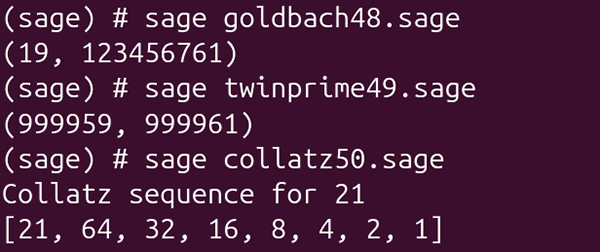
Now, let us execute these three programs and examine their output. Figure 1 shows the output produced when the programs are executed. Verify that each program behaves as expected. Confirm that the pair returned by goldbach48.sage consists of two prime numbers whose sum equals the given even integer, and that the pair returned by twinprime49.sage consists of two prime numbers differing by exactly 2. You may use the SageMath function is_prime( ) to verify the primality of the numbers returned by both programs. Finally, verify that every term in the Collatz sequence generated by collatz50.sage follows the rules of the Collatz Conjecture and that the sequence eventually terminates at 1. With that, we conclude our discussion of number theory.
As this is the final article in this series, let us conclude by taking a brief tour of a few other fields of mathematics and computer science where SageMath excels. Its scope is remarkably broad, encompassing numerous branches of mathematics, engineering, and scientific computing. While it is impossible to cover them all within the confines of this series, it is worthwhile to highlight SageMath’s capabilities in four important areas: numerical analysis, statistics, linear algebra, and calculus.
Numerical analysis
Numerical analysis is concerned with obtaining approximate solutions to mathematical problems that cannot be solved exactly using analytical methods. It plays a vital role in engineering, physics, optimization, finance, weather prediction, machine learning, artificial intelligence, and many other scientific disciplines. SageMath provides a comprehensive environment for numerical computation by integrating several powerful libraries, including GSL (GNU Scientific Library), MPFR, MPFI, Arb, mpmath, SciPy, and NumPy. These libraries enable SageMath to perform high-precision arithmetic, numerical integration, root-finding, optimization, and a wide range of other numerical computations efficiently.
Let us now look at a few SageMath one-liners related to numerical analysis. The function find_root(f, a, b) numerically computes a root of the function f within the interval [a,b]. The function numerical_integral(f, a, b) numerically evaluates the definite integral of f over the interval [a,b]. Unlike symbolic integration, which attempts to derive an exact mathematical expression, numerical integration computes an approximate value using efficient numerical algorithms. The function returns a pair of values: the first is the computed value of the integral, while the second is an estimate of the numerical error. Finally, the function find_local_maximum(f, a, b) numerically determines a local maximum of the function f over the specified interval. It returns a pair consisting of the maximum value of the function and the point at which this maximum occurs. Figure 2 shows the output produced by these SageMath one-liners.
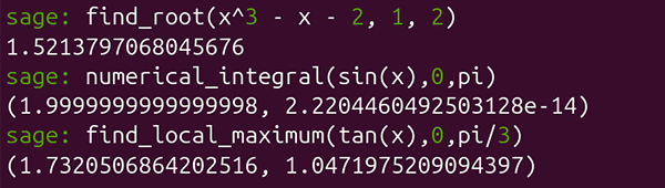
Let us now try to understand the output shown in Figure 2. The output of the function find_root( ) indicates that the equation x3−x−2=0 has a solution in the interval [1, 2] that is approximately equal to 1.52138. Substituting this value into the equation yields a result that is very close to zero, confirming that it is indeed a root of the equation. The output of the function numerical_integral( ) shows that the numerical value of the integral of sin(x) over the interval [0, π] is approximately 1.9999999999999998, which is extremely close to the exact value of 2. The second value in the output is an estimate of the numerical error. Since this value is extremely small (2.2204460492503128×10⁻¹⁴), the computed result is highly accurate. Finally, the output of the function find_local_maximum( ) indicates that the maximum value of tan(x) over the interval [0, π/3] is approximately 1.7320506864, attained at 1.0471975209 radians, which is approximately π/3. Since the tangent function is monotonically increasing over this interval, the maximum naturally occurs at the right endpoint. Consequently, the computed maximum is very close to the exact value, tan(π/3) = √3 ≈1.7320508076.
Statistics
Statistics is the science of collecting, analysing, interpreting, and presenting data. It plays a central role in scientific research, data science, artificial intelligence, finance, healthcare, and numerous other fields where informed decisions are driven by data. SageMath provides a powerful environment for statistical computing by integrating widely used libraries such as NumPy, SciPy, and R, enabling users to perform a broad range of statistical analyses through a unified interface. Let us now look at a few SageMath one-liners for statistical computing, shown in Figure 3. Notice that these one-liners are standard Python statements, once again demonstrating that SageMath seamlessly integrates with the vast Python ecosystem while providing a rich mathematical environment for scientific computing.
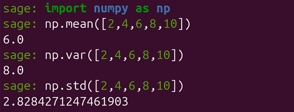
Let us now understand the output produced by these statistical functions. The function np.mean( ) computes the arithmetic mean of the given data. For the list [2,4,6,8,10], the mean is 6.0, which is obtained by dividing the sum of the numbers (30) by the total number of observations (5). The function np.var( ) computes the population variance, which measures how far the observations are spread around their mean. For the given data, the variance is 8.0. Finally, the function np.std( ) computes the population standard deviation, which is the square root of the variance. The output 2.8284271247461903 is approximately equal to √8, indicating the average spread of the observations from the mean. These functions are provided by the NumPy library, which is tightly integrated with SageMath and is widely used for statistical analysis and scientific computing.
Linear algebra
Linear algebra is the branch of mathematics that studies vectors, matrices, and systems of linear equations. It forms the mathematical foundation of modern scientific computing and underpins numerous fields, including computer graphics, optimization, signal processing, robotics, and scientific simulation. In recent years, its importance has grown even further, as much of modern artificial intelligence and quantum computing can be viewed as linear algebra in disguise—from neural network operations and tensor computations to quantum states and quantum gates, the underlying mathematics is fundamentally based on vectors and matrices. SageMath provides an excellent environment for linear algebra by integrating highly optimized libraries such as BLAS, LAPACK, ATLAS, LinBox, and IML, enabling efficient and scalable matrix computations.
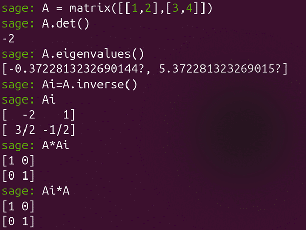
Let us now understand the output produced by the linear algebra functions shown in Figure 4. The function det( ) computes the determinant of a matrix. In this example, the determinant of the matrix A is −2, indicating that the matrix is non-singular (its determinant is non-zero) and hence invertible. The function eigenvalues( ) computes the eigenvalues of the matrix, which are approximately −0.3723 and 5.3723. These values satisfy the characteristic equation of the matrix and have numerous applications in fields such as machine learning, computer graphics, signal processing, and the solution of systems of differential equations. The function inverse( ) computes the inverse of the matrix A, denoted by A−1. Finally, the matrix products A*Ai and Ai*A both yield the identity matrix, confirming that Ai is indeed the inverse of A. This follows directly from the defining property of the inverse of a matrix: AA−1=A−1A=I, where I denotes the identity matrix.
Calculus
Calculus is the branch of mathematics that studies change and accumulation through the concepts of limits, differentiation, and integration. It forms the mathematical foundation of physics, engineering, economics, and countless areas of scientific computing. In recent years, calculus has also become indispensable in artificial intelligence, where derivatives drive optimization algorithms such as gradient descent used to train deep neural networks. Although linear algebra is the primary mathematical language of quantum computing, calculus also plays an important role in areas such as quantum dynamics, differential equations, variational methods, and quantum control. SageMath provides a comprehensive environment for symbolic and numerical calculus by integrating powerful computer algebra systems and numerical libraries, making it an excellent platform for exploring both classical and modern applications of calculus.
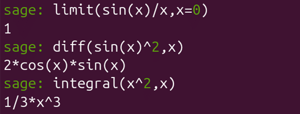
Let us now understand the output produced by the calculus functions shown in Figure 5. The function limit( ) computes the limit of a function as the variable approaches a specified value. In the above example, the output 1 indicates that the limit of sin(x)/x as x approaches 0 is 1; this is one of the most fundamental results in differential calculus, often referred to as the first remarkable limit or the fundamental trigonometric limit. The function diff( ) performs symbolic differentiation. The output 2*cos(x)*sin(x) is the derivative of sin2(x), obtained by applying the chain rule. Finally, the function integral( ) performs symbolic integration. The output 1/3*x^3 is the indefinite integral of x2, indicating that the integral of x2 is x3/3 (up to an arbitrary constant of integration). These examples demonstrate SageMath’s ability to perform symbolic calculus efficiently by leveraging powerful computer algebra systems such as Maxima, SymPy, GiNaC, Giac, and FriCAS.
Beyond the mathematical capabilities explored throughout this series, SageMath also incorporates numerous infrastructure and visualisation components, including SQLite, ZODB, Twisted, MathJax, Matplotlib, Tachyon, GD, and Jmol. These libraries provide essential services such as persistent data storage, networking, high-quality mathematical typesetting, two-dimensional and three-dimensional visualisation, rendering, and interactive user interfaces. Although they operate largely behind the scenes, they are fundamental to SageMath’s architecture, transforming it from a collection of mathematical algorithms into a comprehensive ecosystem for scientific computing.
As we conclude this series, it is worth reflecting once again on why tools like SageMath matter. We live in an era where AI assistants such as ChatGPT and Claude are steadily automating many aspects of conventional programming. Writing boilerplate code and even implementing standard algorithms are becoming increasingly routine tasks. In such a world, the true value lies not merely in the ability to write code, but in understanding the mathematical and scientific principles that underpin modern computing. Scientific computing, symbolic mathematics, optimization, graph theory, cryptography, and related disciplines are therefore becoming more relevant than ever. Tools like SageMath empower us to explore these deeper ideas and transform them into working solutions. While this series may end here, the journey of scientific computing itself is only beginning, and I hope that SageMath will continue to serve as a trusted companion in your explorations.