Quantum Computing: Beyond One Qubit

The central theme of this fourth article in the series on quantum computing is the Controlled-NOT (CNOT) gate, which is a multi-qubit quantum gate.

In the first three articles in this series on quantum computing, we developed an intuitive understanding of the behaviour of a single qubit using tools such as the Bloch sphere simulator. These visualisations helped us explore the action of various quantum gates that operate on a single qubit. We now move beyond single-qubit systems and begin our study of multi-qubit systems and the quantum gates that act on them.

However, before we proceed any further, let us take a brief detour to understand another formidable challenge in quantum computing. Developing an elegant quantum algorithm is only half the battle; the underlying quantum hardware must faithfully execute it. Unfortunately, this hardware exists in an extremely delicate quantum state, making it one of the greatest engineering challenges of our time. So far, our discussions have largely revolved around writing quantum programs and executing them on ideal simulators. Real quantum computers, however, are far from perfect and are susceptible to errors. Throughout this discussion, we shall continue focusing on superconducting quantum computers. In the previous article, we introduced the Josephson junction, the fundamental building block of a superconducting qubit. Let us now build upon that discussion and explore the enormous engineering challenge involved in constructing a superconducting quantum computer. Only then can we truly appreciate why today’s quantum hardware is inherently prone to errors—and why even a brilliantly designed quantum algorithm can fail to deliver the expected results on real hardware.

Unlike a classical bit, which can reliably exist as either 0 or 1 under ordinary operating conditions, a superconducting qubit must preserve an extremely fragile quantum state. Even the slightest interaction with its surroundings—thermal radiation, stray electromagnetic fields, microscopic material defects, cosmic rays, or vibrations from the environment—can disturb this state, causing the qubit to lose the quantum information it is carrying. This process, known as decoherence, is one of the greatest obstacles in the construction of practical quantum computers. In other words, the biggest challenge is not creating a qubit, but keeping it ‘quantum’ long enough to perform meaningful computations.

To overcome these challenges, engineers employ some of the most sophisticated technologies available today. Superconducting qubits are fabricated using advanced nanofabrication techniques and operated inside dilution refrigerators that cool them to temperatures of only a few millikelvin—colder than outer space. Precisely shaped microwave pulses are then used to manipulate individual qubits and implement quantum gates, while elaborate shielding and filtering systems protect them from external noise. Even after all these engineering efforts, present-day quantum processors remain noisy, giving rise to the term Noisy Intermediate-Scale Quantum (NISQ) computers. This explains why running the same quantum program on a simulator and on a real quantum processor often produces noticeably different results.

Now that we understand that present-day quantum hardware is not perfectly reliable, an obvious question arises: how can we imitate the error-prone behaviour of a real quantum computer while developing and testing quantum algorithms? Qiskit provides us with methods to simulate such noisy quantum systems. To understand this, let us revisit the program qiskit4.py, discussed in the second article of this series, which demonstrated the operation of the Pauli-X gate. You may recall that after executing the circuit for 1000 shots, the output was always {1: 1000}. This is because the Pauli-X gate behaves like the classical NOT gate, flipping the initial qubit state from |0 to |1every time it is applied. Since the qubit is measured in a computational basis, the state |1 always produces the classical output 1. The result clearly demonstrates that the simulator assumes an ideal quantum computer, where every gate and every measurement is performed perfectly without any influence of hardware-induced errors.

Now, consider the program qiskit7.py (with line numbers included for clarity), shown below, which artificially introduces errors into the quantum system.

1. from qiskit import QuantumCircuit, transpile

2. from qiskit_aer import AerSimulator

3. from qiskit_aer.noise import NoiseModel, pauli_error

4. qc = QuantumCircuit(1, 1)

5. qc.x(0)

6. qc.measure(0, 0)

7. noise_model = NoiseModel( )

8. error = pauli_error([(“X”, 0.05), (“I”, 0.95)])

9. noise_model.add_all_qubit_quantum_ error(error, [“x”])

10. noisy_sim = AerSimulator(noise_ model=noise_model)

11. compiled = transpile(qc, noisy_ sim)

12. result = noisy_sim.run(compiled, shots=1000).result( )

13. print(result.get_counts( ))

In the program above, the statements used to create the quantum circuit, apply the Pauli-X gate, perform measurements, and execute the circuit on the simulator were explained previously. Therefore, the following discussion focuses only on the newly introduced statements that allow the simulator to model the behaviour of a noisy quantum computer. In addition to importing the class QuantumCircuit, Line 1 imports the function transpile( ). Transpilation is the process of converting a quantum circuit into a form that is compatible with a specific quantum backend. Since we shall be executing the circuit on a noisy simulator configured to imitate a real quantum processor, the circuit must first be transpiled for that backend. Line 2 imports the class AerSimulator. Line 3 imports the class NoiseModel and the function pauli_error( ) from Qiskit’s noise module. The class NoiseModel is used to define a noise model that describes how errors are introduced into the quantum circuit during simulation. The helper function pauli_error( ) creates an error channel based on Pauli operators. In this example, it is used to introduce errors while executing the Pauli-X gate. Lines 4 to 6 create a single-qubit circuit, apply the Pauli-X gate, and measure the qubit.

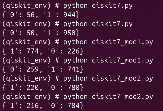
Line 7 creates an empty noise model. At this stage, the model does not contain any errors. Line 8 defines a Pauli error model. The list supplied to the function pauli_error( ) specifies the probabilities associated with different operations: (“X”, 0.05) means that an unwanted Pauli-X error is introduced with a probability of 5% and (“I”, 0.95) means that with a probability of 95%, the identity operation is applied, indicating that no error occurs. Thus, the simulator behaves as though every execution of the gate has a 5% chance of suffering an unwanted Pauli-X error. Line 9 tells the noise model to associate the previously defined error with every Pauli-X gate in the circuit. Consequently, whenever a Pauli-X gate is executed during the simulation, the specified error model is applied automatically. Instead of creating an ideal simulator, Line 10 creates an AerSimulator configured with the noise model defined earlier. As a result, the simulator attempts to imitate the behaviour of a noisy superconducting quantum computer rather than an ideal one. Line 11 transpiles the circuit for a noisy simulator before execution. This step ensures that the circuit is compatible with the target backend and allows the simulator to apply the specified noise model correctly. Line 12 executes the transpiled circuit on the noisy simulator for 1,000 shots and collects the measurement results. Finally, Line 13 displays the measurement statistics. Unlike the ideal simulator, which consistently yields {‘1’: 1000}, the noisy simulator produces probabilistic outcomes such as {‘0’: 56, ‘1’: 944} or {‘0’: 50, ‘1’: 950}. The exact counts vary between runs because errors occur probabilistically. These results help illustrate the imperfect behaviour of real quantum hardware, offering a practical way to analyse noise effects without requiring physical quantum device access.

Now, let us investigate how changing the error probability affects the behaviour of the simulator. To do this, we create two modified versions of qiskit7.py, namely, qiskit7_mod1.py and qiskit7_mod2.py, by replacing Line 8 with error = pauli_error([(“X”, 0.25), (“I”, 0.75)]) and error = pauli_error([(“X”, 0.80), (“I”, 0.20)]), respectively. We shall now execute all three programs and compare their outputs, as shown in Figure 1. Before running the programs, ensure that the virtual environment qiskit_env is activated, just as we did in the previous articles. As the probability of introducing the Pauli-X error increases, the measurement statistics change accordingly. Since the original circuit already applies a Pauli-X gate, an additional Pauli-X error occasionally flips the qubit back to its original state |0. Consequently, increasing the error probability increases the number of measurements that produce 0, while the number of measurements yielding 1 decreases. This simple experiment clearly demonstrates how Qiskit’s noise model can be used to imitate the behaviour of increasingly noisy NISQ-era quantum hardware.

Now comes an important question: How do we decide whether the error probability introduced into our simulator is realistic? Is there a way to benchmark this artificially introduced error against the behaviour of an actual quantum computer? The answer is a resounding ‘Yes’ and, thanks to the technology giant IBM, you can do it free of cost.

In this section, we shall execute a modified version of our original Pauli-X gate program qiskit4.py on an actual superconducting quantum computer made available through the IBM Quantum Platform. The first step is to visit the IBM Quantum Platform portal and create a free account. Fortunately, you do not need a credit card to register, and the free tier provides limited access to real quantum hardware, allowing you to gain hands-on experience with an actual quantum computer. This is an extraordinary opportunity, considering that operating such sophisticated quantum hardware is extremely expensive. Commercial access to quantum computing resources can cost tens of dollars per minute, making IBM’s free offering an invaluable resource for students, educators, researchers, and quantum computing enthusiasts around the world.

When you sign in to your IBM Quantum Platform account, you can select the region in which your instance is located: us-east or eu-de. Note, however, that the Open Plan (free plan) is currently available only in the us-east (Washington, D.C.) region. Once you have signed in, the Home screen provides an option to generate an API key, as shown in Figure 2. You will be prompted to provide a name for the key, after which you can either download it as a JSON file or simply copy it to the clipboard. This API key is then used by the program qiskit8.py, shown below, which applies a Pauli-X gate to a single qubit, just like the program qiskit4.py. The only difference is that qiskit4.py was executed on a simulator, whereas qiskit8.py is executed on an actual superconducting quantum computer. Yes—at this very moment, somewhere in a quantum computing facility in the United States, your Python program instructs one of the most ingeniously engineered machines ever built to generate precisely controlled microwave pulses and perform a genuine quantum computation. How wonderful is that!

from qiskit import QuantumCircuit

from qiskit.transpiler.preset_passmanagers import generate_preset_pass_manager

from qiskit_ibm_runtime import QiskitRuntimeService, SamplerV2 as Sampler

API_KEY=”PasteYourAPIKeyHere”

QiskitRuntimeService.save_account(

channel=”ibm_quantum_platform”,

token=API_KEY,

overwrite=True

)

service = QiskitRuntimeService( )

backend = service.least_busy(operational=True, simulator=False)

print(f”--> Target QPU Selected: {backend.name}”)

qc = QuantumCircuit(1, 1)

qc.x(0)

qc.measure(0, 0)



pm = generate_preset_pass_manager(backend=backend, optimization_level=1)

isa_circuit = pm.run(qc)



sampler = Sampler(mode=backend

job = sampler.run([isa_circuit], shots=1000)

print(f”--> Job Submitted! Job ID: {job.job_id( )}”)

result = job.result( )

pub_result = result[0]

counts = pub_result.data.c.get_counts( )

print(“\nReal Hardware Results:”, counts)

Since the program qiskit8.py does not introduce any new quantum computing concepts and differs from qiskit4.py only in the IBM Quantum Platform-specific code required to execute the circuit on real hardware, I shall not explain it line by line in order to save space. However, notice that the lines of code used to create the qubit, apply the Pauli-X gate, and perform the measurement are identical to those in qiskit4.py.

Before executing qiskit8.py, we must first install the IBM Runtime package. After activating the virtual environment qiskit_env, execute the following command in the terminal: pip install qiskit-ibm-runtime. Next, replace the placeholder API_KEY = “PasteYourAPIKeyHere” in qiskit8.py with the API key obtained from your IBM Quantum Platform account. Simply paste your API key inside the double quotation marks. Once these steps are complete, execute the program on an actual IBM quantum processor by running the command python qiskit8.py from the terminal. The measurement statistics obtained from executing the program on a real IBM quantum computer are shown in Figure 3.

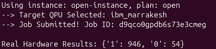
While executing qiskit8.py, you may notice a few warning messages before the actual program output. These are normal and indicate that Qiskit IBM Runtime is automatically selecting an available instance for your account. In our case, the open instance was selected. Since IBM’s quantum processors are shared by users worldwide, Open Plan users may occasionally experience waiting times. Depending on processor availability, IBM automatically selects a suitable backend. In our case, the program was executed on ibm_marrakesh, one of IBM’s latest Heron R2 superconducting quantum processors.

The measurement statistics obtained from the real quantum processor are {‘1’: 946, ‘0’: 54}. In contrast, an ideal simulator always produces {‘1’: 1000} because the Pauli-X gate deterministically transforms the state |0 into |1. The 54 incorrect outcomes clearly demonstrate that present-day NISQ-era quantum hardware is prone to errors arising from imperfections such as gate errors, decoherence, and measurement errors. Fortunately, as demonstrated earlier in this article, Qiskit’s noise models allow us to imitate these hardware imperfections using a simulator.

Interestingly, the real quantum processor produced 0 in 54 out of 1000 shots, corresponding to an error rate of about 5.4%. This is remarkably close to the 5% Pauli-X error probability used in our original noisy simulation. However, we should not conclude that the actual quantum processor has an overall error rate of exactly 5.4%. Our simple noise model represents only one type of error, whereas a real quantum processor is affected by several sources of error, including gate errors, decoherence, and measurement errors. Nevertheless, this comparison gives us useful intuition about how a simple noise model can approximate the behaviour observed on real hardware.

A closer look at Figure 2 reveals several useful details about the IBM Quantum Platform. Besides providing options for managing API keys, the dashboard also displays the available quantum instance (open-instance) and the remaining free usage time, which in our case is 9 minutes and 10 seconds. It also maintains a record of recently executed quantum jobs, showing their execution status, the quantum processor used (ibm_marrakesh), and the execution time for each job.

Now, let us take a small digression and introduce two important notations: the positive X-basis state, denoted by |+(read as ‘ket plus’), and the negative X-basis state, denoted by | – (read as ‘ket minus’), as shown in Figure 4. These states are obtained by applying the Hadamard gate to the computational basis states |0and |1, respectively. You will encounter these notations repeatedly throughout quantum computing, so I strongly recommend committing them to memory. They will soon become your close companions as we continue our journey into the quantum world.

A first look at the CNOT gate

Now, let us add a lot of power to the quantum computing model that we have been patiently developing by adding one more qubit. At first glance, this might look like a simple extension of the programs we have been writing for a single qubit. No! By moving from one qubit to two, we open the door to another fascinating quantum-mechanical phenomenon—entanglement. We have already encountered superposition while working with a single qubit. However, to create entanglement, we need at least two qubits that can interact with each other. Superposition, entanglement, interference, and other quantum-mechanical phenomena form the foundation on which quantum algorithms exploit the laws of quantum mechanics to tackle certain problems in ways that classical algorithms running on today’s digital computers cannot.

It will take more than one article to fully appreciate the fascinating and sometimes rather tricky behaviour of entanglement. In fact, entanglement is arguably one of the most counterintuitive ideas in quantum mechanics. A famous quote often attributed to Niels Bohr goes, “Anyone who is not shocked by quantum theory has not understood it.” The exact wording and attribution of this quote are disputed, so let us not get caught up in that debate just yet! I am sure many of you are already wondering about entanglement and may have encountered some of the myths surrounding it, including the idea of ‘faster-than-light’ communication. Since entanglement is difficult enough to understand as a physical phenomenon, let us leave the deeper mathematical and philosophical discussion for later. Instead, let us dive straight into a program. Consider the program qiskit9.py, shown below, which creates an entangled state involving two qubits using a CNOT gate. The CNOT gate is a two-qubit gate in which one qubit acts as the control and the other as the target. The target qubit is flipped from |0 to |1 or from |1 to |0 only when the control qubit is in the state |1; if the control qubit is |0, the target qubit remains unchanged. In our program, qubit 0 is the control and qubit 1 is the target.

1. from qiskit import QuantumCir cuit, transpile

2. from qiskit_aer import AerSimulator
3. qc = QuantumCircuit(2, 2)

4. qc.h(0)

5. qc.cx(0, 1)

6. qc.measure([0, 1], [0, 1])

7. simulator = AerSimulator( )

8. compiled = transpile(qc, simulator)

9. result = simulator.run(compiled, shots=1000).result( )

10. counts = result.get_counts( )

11. print(counts)

Now, let us try to understand the working of the program qiskit9.py. Line 1 imports the class QuantumCircuit and the function transpile from Qiskit. The function transpile( ) converts the circuit into a form suitable for the selected backend. Line 2 imports the class AerSimulator from the package qiskit_aer. The AerSimulator enables us to execute quantum circuits on a classical computer and observe their measurement outcomes. Line 3 creates a quantum circuit containing two qubits and two classical bits. Line 4 applies the Hadamard gate to qubit 0, putting it into an equal superposition of |0 and |1 (the |+state). Line 5 applies the Controlled NOT (CNOT) gate, with qubit 0 as the control and qubit 1 as the target. Together, Lines 4 and 5 transform the initial state |00 into the entangled Bell state (|00+|11)/√2. Line 6 measures both qubits and stores their measurement results in the corresponding classical bits. Thus, the measurement result of qubit 0 is stored in classical bit 0, while that of qubit 1 is stored in classical bit 1. Line 7 creates an instance of the AerSimulator and assigns it to the variable simulator. Line 8 transpiles the quantum circuit so that it is compatible with the selected simulator. Line 9 executes the transpiled circuit on the simulator for 1000 shots and stores the resulting data. Line 10 extracts the measurement statistics from the variable result and stores them in the variable counts. Finally, Line 11 prints these statistics on the screen. Since we are using an ideal simulator, the output will typically contain only 00 and 11, with approximately 500 occurrences of each. This striking correlation between the measurement outcomes of the two qubits is our first glimpse of the fascinating phenomenon of quantum entanglement.

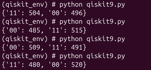
Now, let us execute the program qiskit9.py and understand its output. Figure 5 shows the results of four successive executions of the program qiskit9.py. The measurement statistics obtained are {‘11’: 504, ‘00’: 496}, {‘00’: 485, ‘11’: 515}, {‘00’: 509, ‘11’: 491}, and {‘11’: 480, ‘00’: 520}, respectively. We know that when two independent qubits are measured, there are four possible outcomes: 00, 01, 10, and 11. However, the two qubits in our circuit are entangled and are therefore not independent of each other. If qubit 0 is measured as 0, qubit 1 will also be measured as 0 with certainty. Similarly, if qubit 0 is measured as 1, qubit 1 will also be measured as 1 with certainty. Consequently, the only possible measurement outcomes are 00 and 11. Since qubit 0 has an equal probability of being measured as 0 or 1, we obtain approximately equal numbers of 00 and 11 outcomes over 1000 shots. The small variations in the counts across the four executions are simply a consequence of the probabilistic nature of quantum measurement.

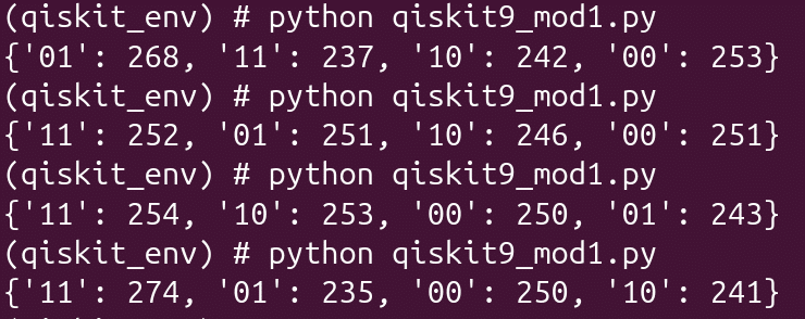
Let us now slightly modify the program qiskit9.py to see what happens when the two qubits are not entangled. The program qiskit9_mod1.py is obtained by replacing Line 5 with qc.h(1). Here, instead of using a CNOT gate to entangle the two qubits, we apply a Hadamard gate independently to qubit 1 as well. Figure 6 shows the results of four successive executions of qiskit9_mod1.py. As we can see from the figure, all four possible combinations—00, 01, 10, and 11—occur with approximately equal probability, with roughly 250 occurrences of each in 1000 shots. This is exactly what we would expect when the two qubits are independent. So, for this circuit, the moral of the story is simple: no CNOT, no entanglement!

Now, let us do some myth busting. Is it possible to communicate faster than light using entangled particles? Let us consider a theoretical scenario. You and your friend share a collection of entangled qubit pairs and then travel light years apart. You measure your qubit and suppose you obtain 1. If your friend measures the other qubit in the same computational basis, he will also obtain 1 with certainty. It may therefore appear that you have somehow communicated the result of your measurement instantaneously. But have you actually sent any information faster than light? The answer is a big ‘No’.

Suppose you want to send a single bit of information—say, 0—to your friend. You cannot force your entangled qubit to produce 0 when measured. The outcome is fundamentally random. You could keep measuring identically prepared entangled pairs until you happen to obtain 0, but your friend has no way of knowing which pair produced that result. Suppose, for example, that you share five entangled pairs. You measure the first two pairs and obtain 1, while the third measurement gives you the 0 you wanted to communicate. Here comes the catch: how will you tell your friend that the third pair is the one he should examine? You must send that information through a classical communication channel, and classical information cannot travel faster than light. Your friend can therefore discover the correlation only after receiving information through an ordinary communication channel. Thus, although entanglement produces correlations that cannot be explained by classical physics, it cannot be used for faster-than-light communication. Faster-than-light communication through entanglement is therefore a science-fiction plot device, not a feature of quantum mechanics.

Now, it is time to conclude our discussion. In this article, we saw how a quantum computing simulator can be configured to imitate some of the noisy behaviour of a real quantum processor. We then took a step further by executing a quantum program on an actual superconducting quantum computer through the IBM Quantum Platform. Finally, we shifted our gears from the world of single qubits to the exciting realm of multi-qubit systems, where we encountered the CNOT gate and the fascinating phenomenon of quantum entanglement. These concepts open the door to the truly quantum world of computing, where the real power of quantum systems begins to unfold. In the next article in this series, we will delve deeper into entanglement, explore Bell states and related concepts, and take a closer look at the various sources of errors that affect today’s superconducting quantum computers.