
























































This series on quantum computing aims to equip beginners with a strong conceptual foundation and gradually guide them towards an intermediate-level understanding of quantum computing, enabling them to participate confidently in this emerging tech revolution.
The year 2025 was observed by the United Nations as the International Year of Quantum Science and Technology (IYQ) to commemorate one hundred years of quantum mechanics. The quantum era began with the publication of the celebrated research paper known as the ‘Umdeutung’ paper by the renowned physicist and Nobel laureate Werner Heisenberg. Over the past century, quantum mechanics has influenced nearly every aspect of modern life by providing the scientific foundation for technologies such as semiconductors, integrated circuits, MRI scanners, lasers, electron microscopes, and GPS systems. Yet, it is quite possible that the greatest technological achievement enabled by quantum mechanics is still to come: the quantum computer.
Interest in quantum computing has grown dramatically in recent years, supported by substantial investments from both technology companies and governments around the world. The emergence of quantum machine learning has further strengthened the case for developing scalable and reliable quantum hardware. Major technology companies—including IBM, Google, Microsoft, NVIDIA, and Meta—are investing heavily in quantum technologies and related research.
The government of India launched the National Quantum Mission (NQM) in April 2023 under the Department of Science and Technology to accelerate the development of quantum technologies in the country. Many other nations are also investing heavily in quantum computing. This global surge of interest is hardly surprising. It is widely believed that the first nation to develop a large-scale, fault-tolerant quantum computer could gain a substantial strategic and technological advantage. This is similar to the military advantage of a country that alone possesses nuclear weapons. It is easy to see that such a nation would wield enormous influence and effectively dictate the rules of the world.
This brings us to an important question for students of science and technology, as well as IT professionals: should we strive to become early adopters who help shape the future of quantum computing, or should we wait and follow developments led by others?
Many existing tutorials treat quantum programming as just another programming subject, focusing mainly on writing code while paying little attention to the mathematics behind the code or the hardware that ultimately executes it. The distinctive feature of this series is its three-level approach to understanding quantum computing:
- The coding level — what happens when a particular line of quantum code is written.
- The mathematical level — the linear algebra and quantum mechanics that explain and justify that line of code.
- The hardware level – the physical processes taking place inside an actual quantum processor when the code is executed.
By examining quantum computing from these three perspectives, you can gain a deeper and more complete understanding of how quantum computers work.
Several important tools and platforms used in quantum computing will be introduced in this series on quantum computing. We will begin with Qiskit, a Python-based, free and open source software development kit (SDK) for quantum computing developed by IBM. We will then move on to OpenQASM (Quantum Assembly Language), an intermediate representation for quantum circuits that enables the low-level description and execution of quantum programs. Next, we will explore Cirq, a free and open source Python framework developed by Google for designing and simulating quantum circuits, with a strong focus on near-term quantum devices. From there, we will proceed to Q#, a domain-specific quantum programming language developed by Microsoft for building quantum algorithms integrated with classical control. Q# is also free and open source and is distributed under the MIT License. In addition, we will become familiar with Qniverse, an indigenously developed quantum computing platform created by C-DAC in India.
There are many misconceptions and myths surrounding quantum computing. As we progress through this series, we will attempt to clarify and dispel several of them. Some of the important questions that will be addressed include the following: Will quantum computers eventually replace classical computers entirely? Does faster code execution in quantum computing depend solely on parallelism, as in GPUs or TPUs? Do qubits allow exponential storage of information through superposition? Does quantum entanglement enable faster-than-light communication?
Finally, although the focus of the series is quantum computing, we will also briefly explore related areas such as quantum communication and quantum sensing. Topics such as Quantum Key Distribution (QKD) and Post-Quantum Cryptography (PQC) will be discussed in the context of secure communication. In addition, we will touch upon emerging topics in quantum sensing, which exploit quantum phenomena to achieve extremely precise measurements. Together, these discussions will give you a broad and comprehensive understanding of the rapidly evolving landscape of quantum technologies.
A brief history of quantum computing
Let us begin with the scientist most often credited with proposing the idea of quantum computing: Richard Feynman, the brilliant physicist and Nobel laureate. Feynman realised that classical computers cannot efficiently simulate quantum mechanical systems because the computational resources required grow exponentially with the size of the quantum system. In the early 1980s, he proposed that computers based on the principles of quantum mechanics could overcome this limitation. Such machines would exploit uniquely quantum mechanical phenomena such as superposition, entanglement, and interference. Around the same time, the Russian mathematician Yuri Manin independently suggested the possibility of a computing model based on quantum mechanics. For this reason, both Richard Feynman and Yuri Manin are often credited with laying the conceptual foundations of the quantum computer.
Although we will not discuss complex quantum algorithms in detail in this article, it is important to mention two algorithms that ensured the survival and growth of the idea of quantum computing. While quantum computers were originally proposed to simulate quantum systems, there were initially no practical algorithms demonstrating clear advantages over classical computing. This situation changed dramatically in 1994, when Peter Shor introduced the famous Shor’s algorithm.
Shor’s algorithm showed that a sufficiently powerful quantum computer could efficiently factor large integers. This result has profound implications for modern cryptography, because many widely used public-key cryptosystems rely on the difficulty of integer factorisation. For example, the RSA cryptosystem, which underlies many secure communications and financial transactions, could be broken if a large-scale quantum computer becomes available. Such a development would have significant consequences for global cybersecurity and the world economy.
Another important milestone came in 1996, when Lov Grover, an Indian computer scientist, introduced Grover’s algorithm. This algorithm provides a quadratic speedup for searching an unstructured database, making it significantly faster than classical search methods. Later, it was proven that this quadratic speedup is the best possible for unstructured search, ensuring that Grover’s algorithm remains one of the most important works in quantum computing.
Together, these two algorithms demonstrated that quantum computers could have practical applications beyond the simulation of quantum systems. They showed that quantum computing could potentially transform fields such as cryptography, optimisation, and data processing, ensuring that the concept of quantum computing would evolve from a theoretical curiosity into a serious area of research.
Understanding the qubit
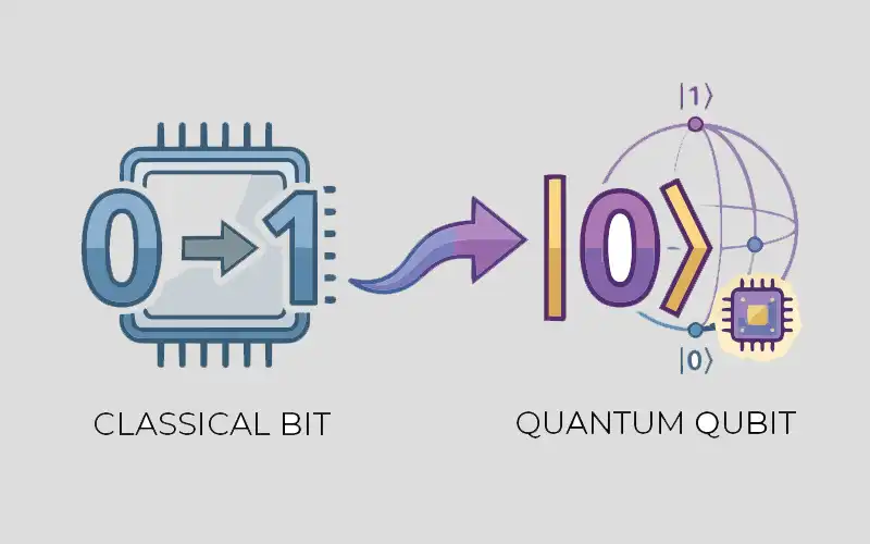
Now it is time to begin our technical discussion of quantum computing. The basic unit of quantum information is the qubit. It may be thought of as the quantum counterpart of the classical bit, the fundamental unit of information in a digital computer. However, the similarity between a bit and a qubit ends there.
A classical bit can store only one of two possible values: 0 or 1. A qubit, on the other hand, can exist in the state |0 (read as ‘ket zero’), |1 (read as ‘ket one’), or in a superposition of these two states. This idea also explains the title of this article, ‘From Zero to Ket Zero’.
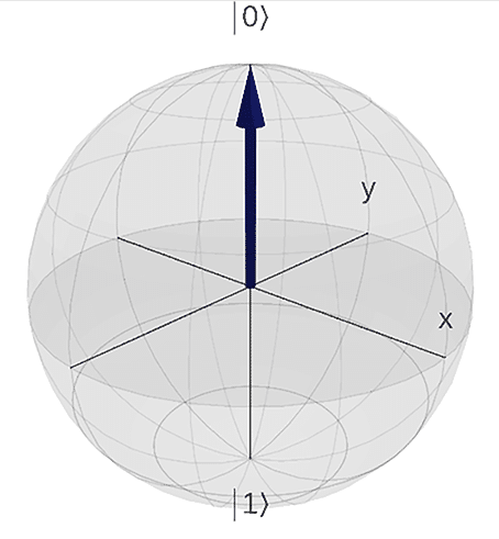
For visualisation and study purposes, the state of a single qubit can be represented using the Bloch sphere, which is named after the physicist Felix Bloch, another Nobel laureate. Figure 1 shows the Bloch sphere representation of the state 0. The figure was generated using the Bloch sphere simulator available at https://bloch.kherb.io/, which is distributed under the MIT License. This simulator is a useful tool for studying the effect of various quantum gates on a single qubit. It should be noted that the Bloch sphere representation works only for single-qubit systems. When more than one qubit is involved, the state of the system exists in a much higher-dimensional space, making a simple geometric representation like the Bloch sphere impossible.
Now let us try to understand the value stored in a qubit. Before proceeding further, it is worth recalling a famous remark by Richard Feynman, which highlights the conceptual difficulty of quantum mechanics. Feynman once said, “I think I can safely say that nobody understands quantum mechanics.” This statement reflects the inherent complexity of the subject and explains why, even today, relatively few people work in fields such as quantum computing.
Returning to our technical discussion, the state of a single qubit can be visualised using the Bloch sphere. In this representation, the state |0 corresponds to the north pole of the Bloch sphere (see Figure 1), while the state |1 corresponds to the south pole. However, the most important aspect of a qubit is that it can also exist in a superposition of these two states. In general, the state of a qubit can be written as |ψ=α|0+β|1 where α and β are complex numbers known as probability amplitudes. These amplitudes satisfy the normalization condition |α2+|β2=1. Here, |α2 represents the probability of measuring the state |0, while |β2 represents the probability of measuring the state |1. For example, consider the qubit state |ψ=√(1/2)|0+√(1/2)|1 = √(1/2)(|0+|1). In this case, the probabilities of measuring |0 and |1 are both 1/2 because |α|2=|β|2=(√(1/2))2=1/2. We will explore these concepts in greater detail in later articles.
Now, let us take a moment to understand complex numbers, which play a central role in quantum computing. A complex number is a number of the form z=a+bi, where a and b are real numbers, and i is the imaginary unit defined by i2=−1. Complex numbers allow us to represent quantities that have both magnitude and phase, which are essential in describing quantum states and their evolution.
Now a word about the notation |0, ∣|1, and |ψ. This notation is known as bra–ket notation, or Dirac notation, and was introduced by the physicist and Nobel laureate Paul Dirac. As you may have already noticed, the story of quantum computing involves many Nobel Prize–winning physicists.
Two mathematical fields are particularly important for understanding quantum computing: linear algebra and probability theory. Throughout this series, we will cover the necessary mathematical concepts whenever possible. In cases where a detailed explanation is not feasible, the required topics will be clearly indicated so that you can study them separately.
For example, we have already briefly discussed complex numbers, which play a central role in quantum computing. As we move forward, it will also be essential to understand concepts related to matrices and matrix operations. In particular, familiarity with matrix multiplication will be necessary to follow some of the upcoming discussions. If you are not comfortable with these topics, it may be helpful to review them before proceeding further. The Wikipedia article titled ‘Matrix (mathematics)’ is a good starting point for learning about matrices and their properties.
In quantum computing, the state of a qubit is represented using complex probability amplitudes. This means that the coefficients appearing in the expression for a qubit state are complex numbers. For example, the two basic states of a qubit, |0 and |1, can be represented using vectors whose entries are complex numbers. In vector form, these basis states are written as |0=[1 0]T and |1=[0 1]T. These two vectors form the computational basis for a single qubit. Any general qubit state can be expressed as a linear combination of these two basis states with complex coefficients.
Recall from twelfth-standard mathematics that a row vector is a matrix with a single row, while a column vector is a matrix with a single column. The transpose of a row vector A, denoted by AT, is a column vector , and the transpose of a column vector is a row vector.
Now let us turn our attention to quantum gates. Before proceeding further, it is important to note that quantum gates are fundamentally different from the classical logic gates used in present-day digital computers. In simple terms, classical gates are not reversible, whereas quantum gates are reversible. To understand this difference, let us consider a classical gate widely used in digital computers: the AND gate. Figure 2 shows the truth table of AND gate with two input bits.
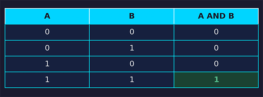
From the figure it is easy to see that the operation of the AND gate cannot be reversed. For example, if the output of an AND gate is 0, there is no way to uniquely determine the exact values of the input bits A and B. The only conclusion we can draw is that the case A=1 and B=1 did not occur. A quantum gate, on the other hand, is reversible. If the same quantum gate is applied twice, we obtain the original state again. This is possible because a quantum gate performs a reversible transformation of the quantum state, typically represented mathematically by a unitary matrix acting on the qubit. At this point, I am sure that the previous sentence may have sounded a bit intimidating and might even have dampened your enthusiasm for learning quantum computing. But do not worry—we will gradually unpack ideas like these in the coming articles in this series. By the end of the series, statements like this will no longer seem mysterious or frightening.
Let us now consider one of the most important quantum gates called the Hadamard gate and study its effect on a qubit. The Hadamard gate is named after the famous French mathematician Jacques Hadamard, who studied the properties of Hadamard matrices. Let us see what happens when a Hadamard gate is applied to a qubit in the state |0. As discussed earlier, the state |0 can be represented by the vector [1 0]T. Similarly, the state |1 can be represented by the vector [0 1]T. A Hadamard gate acting on a single qubit is represented by a special matrix called the Hadamard matrix, denoted by H. The Hadamard matrix H is shown in Figure 3. In this article, we will focus only on the mathematical operation that occurs when a Hadamard gate is applied to a qubit in the state |0.

From Figure 3, we can see that after applying the Hadamard gate, the value of the qubit changes from |0 to √(1/2)|0+√(1/2)|1. Notice that the only mathematical operations involved in the calculations shown in Figure 3 are matrix multiplication and matrix addition. Recall that we previously established that a qubit in the superposition state |ψ=√(1/2)(|0+|1) has an equal probability of being measured as |0 or |1. Thus, the Hadamard gate serves as one of the most important building blocks of quantum circuits, as it creates superposition.
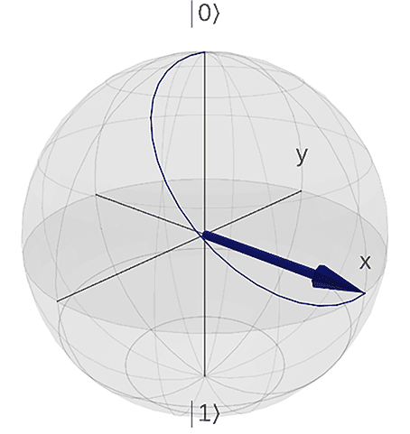
Now let us examine the physical interpretation of applying a Hadamard gate using the Bloch sphere representation. From Figure 1, we know that a qubit in the state |0 is represented by an arrow pointing towards the north pole of the Bloch sphere. Let us again use the Bloch sphere simulator mentioned earlier to observe the effect of the Hadamard gate.
In the Bloch sphere simulator web page, there is a menu labelled ‘Quantum gates’, which includes an option to apply the Hadamard gate. When the Hadamard gate is applied, the Bloch sphere configuration shown in Figure 4 is obtained. From Figure 4, we can see that the state of the qubit now points toward the positive x-axis. It can also be observed that the qubit state is now equidistant from the north and south poles of the Bloch sphere. This observation confirms our earlier calculation: a qubit in the state |ψ=√(1/2)(|0+|1) will produce the outcomes |0 or |1 with equal probability (50–50) upon measurement. Now apply the Hadamard gate a second time, and you will observe that the state of the qubit is represented by an arrow pointing to the north pole of the Bloch sphere. This indicates that the value of the qubit has returned to |0, thereby demonstrating that quantum gates are reversible.
Though we have only seen the effect of the Hadamard gate on a single qubit so far, I would like to make an important statement about the working of quantum gates that provides deep insight into how quantum algorithms operate: all quantum gates correspond to unitary matrix operations acting on state vectors, while measurement is a non-unitary operation. I know that this may sound like another intimidating statement. However, let me repeat my promise: in the next article itself, we will shed much more light on this idea and make the statement far less mysterious.
Installing Qiskit
Now let us begin our hands-on exploration of quantum computing by installing Qiskit, one of the most popular quantum software development kits (SDKs). Qiskit is a Python-based SDK developed by IBM for creating and running quantum circuits.
There are several ways to use Qiskit. However, one of the most operating system–agnostic and convenient approaches is to install it using Anaconda or Miniconda. Anaconda is a full Python distribution that includes many scientific computing packages. It typically requires about 2GB to 3GB of storage space. Miniconda, on the other hand, is a lightweight installer that provides only the conda package manager and Python, requiring about 400MB to 500MB of storage space.
To install Anaconda on Ubuntu, download the installer from the official website and run the following command in the terminal: bash Anaconda3-latest-Linux-x86_64.sh. Note that, at the time of writing this article, the latest version of Anaconda installer for Linux is Anaconda3-2025.12-2-Linux-x86_64.sh. To install Miniconda, download the installer from the official website and run the following command in the terminal: bash Miniconda3-latest-Linux-x86_64.sh. Depending on your storage space and requirements, you may choose either Anaconda or Miniconda for your system.
After installing Anaconda or Miniconda, the next step is to create a virtual environment. This step is important because the version of Python used in the environment matters when installing Qiskit. The versions of Python that work well with the latest version of Qiskit are Python 3.9, 3.10, 3.11, and 3.12. For most users, it is safest to use Python 3.10 or Python 3.11, as these versions are widely tested and stable.
Run the following commands in the terminal to create a virtual environment called qiskit_env, activate it, and install Qiskit. The final command will display the version of Qiskit installed on your system. In my system, the installed version of Qiskit is 2.3.0.
conda create -n qiskit_env python=3.11
conda activate qiskit_env
pip install qiskit
python -c “import qiskit; print(qiskit.__version__)”
Our first quantum program
Now let us execute our first quantum program. The Python program titled ‘qiskit1.py’ (line numbers included for clarity) creates a single qubit and applies a Hadamard gate to it. We are not measuring the value of the qubit at this stage because we will first discuss the theoretical aspects of quantum measurement in detail before performing any measurement operations.
1. from qiskit import QuantumCircuit
2. qc = QuantumCircuit(1)
3. qc.h(0)
4. print(qc.draw( ))
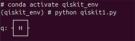
Now let us try to understand how the program works. Line 1 imports the class QuantumCircuit from the library Qiskit. The class QuantumCircuit is used to create and manipulate quantum circuits, which are sequences of quantum operations (gates) applied to qubits. Line 2 creates a quantum circuit containing one qubit and assigns it to the variable qc. The number 1 indicates that the circuit has one qubit. When a qubit is created, it is initialised in the state |0 by default. Thus, at this stage the circuit contains a single qubit in the state |0. Line 3 applies a Hadamard gate to qubit 0 (the first qubit in the circuit). Here, h represents the Hadamard gate, and 0 is the index of the qubit on which the gate is applied. We have already discussed the mathematical operations and physical interpretation of the Hadamard gate. Line 4 generates and prints a visual representation of the circuit. When the program ‘qiskit1.py’ is executed, the output shown in Figure 5 is obtained.
In this article, we have outlined the agenda for the series and introduced some of the fundamental ideas of quantum computing, including the concept of qubits and the basic working of quantum gates. In the next article, we will explore additional quantum gates, examine their properties, and understand how measurement is performed on a qubit to extract information from a quantum system. We will also continue our journey into quantum programming with Qiskit, where we will begin building and experimenting with simple quantum circuits.