


The machine learning landscape is filled with a large number of libraries, each of which comes with its own pros and cons. Choosing the right tool for your application is an important decision. This article explores Flux – a Julia library that provides you the right mix of abstraction and fine-tuning. Flux is fully written in Julia and comes with prominent features such as excellent GPU support and differentiable programming.
Machine learning has evolved into a prominent paradigm of developing solutions to problems. It has enabled solving problems that were earlier unsolvable with relative ease. In the machine learning domain there are plenty of tools and libraries to choose from. Selection of the right tool contributes to the success of the application in a significant manner.
Each of the libraries associated with machine learning has its own advantages and disadvantages. Some of the libraries allow you to work at only the given level of abstraction. If you want to perform some sort of tweaking under the hood to optimise preformance, these libraries make it either very difficult or near impossible.
In this backdrop, Flux is an elegant machine learning stack which is fully written in Julia. If you are absolutely new to Julia, feel free to explore the earlier articles on Julia in this magazine. In a nutshell, Julia is a language that walks like Python and runs like C. It has the advantages of both Python (by making the implementation simpler) and of C (by making the code run faster).
Being fully written in Julia, Flux is guaranteed to run at comparatively greater speed than its counterparts. Another big advantage is that it allows you to work at a great level of abstraction if you wish to do so. At the same time, if you want to go under the hood and tweak the algorithm, it enables you to do so as well. In the words of the official documentation, Flux makes the easy thing easy while remaining fully hackable (https://fluxml.ai/).
The Flux features
Flux comes loaded with features, which as a machine learning engineer you would always prefer to have (Figure 1).
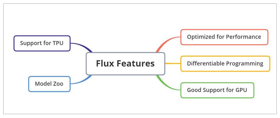
- Optimised for performance.
- Ability to perform differentiable programming. It has state-of-art models such as Neural ODE and Zygote. Automatic differentiation (AD) in Flux can be achieved through its advanced system called Zygote. Computing gradients can be done effortlessly and optimally with Flux.
- Good support for GPU, which is accomplished through CUDA.jl. It comes with fully tweakable support.
- Model Zoo provides a great collection of Flux scripts, which can be utilised to customise as per your needs. Pretrained Flux models are also available with TextAnalysis and Metalhead.
- Support for TPU is an important feature of Flux.
The Flux ecosystem
One of the critical factors that will push you to choose Flux over other tools is the availability of an ecosystem which is very diverse in nature.
- With the help of libraries such as Turing.jl, Bayesian inference and Gaussian processes can be handled on top of Flux.
- Geometric deep learning, which is gaining a lot of attention these days, can be performed through GeometricFlux.
- For computer vision tasks, Metalhead shall be utilised. In the case of transfer learning, these models are highly useful.
- The transformers.jl is adapted for transformer models for natural language processing (NLP) tasks.
Getting started with Flux
Make sure that Julia is installed in your system. The Julia version should be at least 1.3. You can then install Flux with the following simple command in the Julia REPL:
julia> ] add Flux
An alternative method is as shown below:
julia> using Pkg; Pkg.add(“Flux”)
The Flux model Zoo
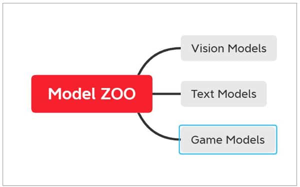
The Flux model Zoo contains a diverse demonstration of Flux. It can be adapted for the objective of your applications as well. The models provided by Flux Model Zoo can be grouped into the following categories:
- Vision models (These are very large convolutional neural networks or CNNs.)
- Text models (though various recurrent neural networks or RNNs)
- Games (through reinforcement learning)
Complete details on the model Zoo can be obtained by navigating to https://github.com/FluxML/model-zoo
Steps involved
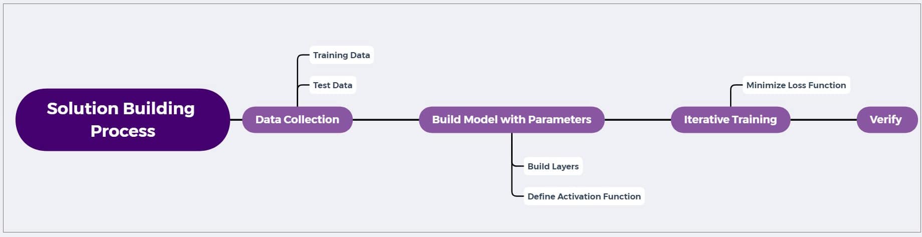
This section explores the steps involved in building a solution through Flux.
- Provide training and test data
- Construct a model with hyper parameters
- Iterative training of the model to improve performance
- Verification of the model
As stated earlier, a significant advantage of Flux is that it enables you to choose the abstraction level. If you prefer to perform each step yourself, then too Flux makes it simple enough to do so. In this section, we will go through building and training a model using Flux in a step-by-step manner. The model will predict the output of the function 2x + 3. The objective of this example is to introduce the steps, more than the actual output.
using Flux
actual(x) = 2x + 3
x_train, x_test = hcat(0:5...), hcat(6:10...)
y_train, y_test = actual.(x_train), actual.(x_test)
Here, the function is coded, and the training and test data are built. Usually, in a real-time scenario, the training and test data will be gathered and cleaned with expert assistance. As we are demonstrating the capability, we have generated the data using the function. The output is as shown below:
([3 5 … 11 13], [15 17 … 21 23])
Let’s build a model:
# Building the model
model = Dense(1, 1)
The model variable will now contain the fields weight and bias. The values of these can be obtained by model.weight and model.bias. The models here are the predictive functions.
predict = Dense(1, 1)
Along with these values, the Dense(1,1) will also implement the function σ(Wx+b). It can be noted that Julia enables naming of functions with Greek letters as well, to match with the equations in the research papers, etc. For example, the following is a Sigmoid function:
σ(1)
0.7310585786300049
If you try the predictions without training, it will obviously make incorrect predictions. So, the next step is to provide a loss function. The loss function informs the Flux how well the model is doing. It does so by computing the cumulative difference between the actual and the predicted values.
loss(x, y) = Flux.Losses.mse(predict(x), y)
loss(x_train, y_train)
In the aforementioned code, MSE stands for Mean Squared Error. The objective of training is to reduce the loss with training.
using Flux: train!
opt = Descent()
data = [(x_train, y_train)]
parameters = params(predict)
train!(loss, parameters, data, opt)
Loop the training by iterating through the data set with the following code snippet:
for epoch in 1:200
         train!(loss, parameters, data, opt)
 end
loss(x_train, y_train)
After the iterative process, the value of loss can be observed as a smaller value. In your implementation, the actual value might differ. But the point here is that it will be a very small one (near zero).
0.0041534975f0
The results can be verified as follows:
The results can be verified as follows:

predict(x_test)
1×5 Matrix{Float32}:
 15.124  17.1438  19.1635  21.1833  23.203

y_test
1×5 Matrix{Int64}:
 15  17  19  21  23
It can be observed from the aforementioned snippet that the predicted values are almost equal to the actual output. This proves that our model has trained well to predict the output of the function that we have given in the beginning.
The models can be constructed by combining various layers (chaining), as shown below:
model2 = Chain(
  Dense(10, 5, σ),
  Dense(5, 2),
  softmax)
Taking gradients
Computing gradients is at the core of many of the ML approaches. Flux enables this computation process to be very effective and optimal. The differentiation can be carried out as follows:
using Flux
f(x) = 3x^2 + 2x + 1;
df(x) = gradient(f, x)[1]; # df/dx = 6x + 2
df(4)
When a function has many parameters, the gradient for each can be computed as follows:
f(x, y) = sum((x .- y).^2);
x = [2, 1];
y = [2, 0]
gs = gradient(params(x, y)) do
         f(x, y)
     end
gs[x]
The output is a vector, as shown below:
gs[x]
2-element Vector{Int64}:
 0
 2
Adding a regularisation term
In machine learning, regularisation is a technique to handle overfitting. Overfitting is a problem when your model performs well with the training data but fails when exposed to novel data. The problem here is the lack of generalisation. There are various regularisation techniques. Flux enables adding regularisation terms very simply. A code snippet is as follows:
m = Chain(
  Dense(28^2, 128, relu),
  Dense(128, 32, relu),
  Dense(32, 10))

sqnorm(x) = sum(abs2, x)

loss(x, y) = logitcrossentropy(m(x), y) + sum(sqnorm, Flux.params(m))

loss(rand(28^2), rand(10))
In the aforementioned example, L2 regularisation is applied by taking the squared norm of the parameters.
GPU support
Flux has good support for GPUs. This can be achieved using CUDA. The CUDA.CuArray shall be used for this purpose. A sample code segment is as shown below:
using CUDA
W = cu(rand(2, 5)) # a 2×5 CuArray
b = cu(rand(2))
predict(x) = W*x .+ b
loss(x, y) = sum((predict(x) .- y).^2)
x, y = cu(rand(5)), cu(rand(2)) # Dummy data
loss(x, y)
GeometricFlux
As stated earlier, GeometricFlux is a geometric deep learning library for Flux. The handling of geometric deep learning using this library can be done similar to handling the traditional models, as shown below:
model = Chain(GCNConv(fg, 1024 => 512, relu),
              Dropout(0.5),
              GCNConv(fg, 512 => 128),
              Dense(128, 10))
## Loss
loss(x, y) = logitcrossentropy(model(x), y)
accuracy(x, y) = mean(onecold(model(x)) .== onecold(y))


## Training
ps = Flux.params(model)
train_data = [(train_X, train_y)]
opt = ADAM(0.01)
evalcb() = @show(accuracy(train_X, train_y))

Flux.train!(loss, ps, train_data, opt, cb=throttle(evalcb, 10))
This article has provided a simple introduction to Flux, which is fully built in Julia. The support for automatic differentiation and GPU will help you to explore Flux for your projects.


